Retrieving initial capital distributions from panel data

Munich Personal RePEc Archive

Retrieving initial capital distributions

from panel data

Chen, Xi and Plotnikova, Tatiana

STATEC/ANEC, 13 rue Erasme, B.P. 304 L-2013 Luxembourg

10 September 2014

Retrieving initial capital distributions from panel data

Xi Chen∗

and Tatiana Plotnikova∗

This version: September 10, 2014

Abstract

A common problem in the empirical production analysis at the firm-level is that the initial values of capital are often missing in the data. Most empirical studies impute initial capital

according to some ad hoc criteria based on a single arbitrary proxy. This paper evaluates

the bias of production function estimations that is introduced when these traditional initial value approximations are used. We propose a generalized framework to deal with the missing initial capital problem by using multiple proxies where the choice of proxies is data-driven. We conduct a series of Monte Carlo experiments where the proposed method is tested against traditional approaches and apply the method to the firm-level data.

Keywords: capital stock measurement, production function estimation, Monte Carlo simu-lation, non-linear regression.

JEL Classification: D20, C19, C81.

∗

STATEC/ANEC, 13 rue Erasme, B.P. 304 L-2013 Luxembourg. [email protected];

[email protected].

1

Introduction

Capital measurement is essential in many fields of economics including growth accounting, pro-duction and productivity analysis. Although the notion of capital input appears quite frequently in economic studies, the questions of what is capital input and how should it be measured oc-cupy economists for decades and still do not have direct answers (Hicks,1974). The main capital measurement issues addressed in the literature include: the evaluation of capital asset efficiency, retirement and user cost (Jorgenson,1963;Hulten,1991;Triplett,1998); the aggregation of het-erogeneous capital (Diewert,1980); the relationship between capital stocks and capital services (Berndt and Fuss,1986) and the link between capital input and production technology (Leontief,

1947; Solow et al., 1960; Fisher, 1965).1 _{While these issues are very important, one practical}

question in capital measurement, the problem of missing initial capital, has not received as much attention. In this paper, we evaluate the implications of missing initial capital in the context of production analysis and propose a framework that generalizes traditional methods of initial value approximation. The proposed method is applicable to micro-level data and is free from ad hoc assumptions of traditional approximation methods.

Production analysis is essentially the study of process that combines different inputs to produce outputs. Typically, input variables in the production process are labour, capital and intermediate materials. While the quantity and price of some inputs are directly available in firms’ records, the data for other inputs are not. For example, the labour service that embodies the labour input, is often measured as total person hours worked. The direct analogy of labour service for capital is capital service measured as total machine hours worked. Unfortunately, the latter information is not available in most production data sets. Researchers usually assume that the capital service is proportional to the productive capital stock, which can be measured. The most used approach to calculate the productive capital stock is the perpetual inventory method (henceforth, PIM), which is based on historical records of investment flows. Following this method, the current capital stock is the weighted sum of an initial capital stock and subsequent investment flows.

One implementation problem of the PIM is that the initial value of capital stock is unob-served. When long series of investment flows are available, the initial condition of the PIM can be set sufficiently far back in the past, so that the initial capital stock is relatively small with respect to the sum of subsequent investment flows. In this case, the problem of missing initial value may play a rather unimportant role. However, production data set that has a long series of investment is rare in practice. At the aggregate level, only few countries have historical data with several decades of investment records. At the disaggregate level, investment data are often limited to few observation points. For the pure time series analysis, the mismeasurement of initial value has a limited impact on the analysis of dynamics. However, when cross-sectional variation is added to the econometric exercise, such as in a panel data regression, the distribution

1

of initial capital stock may have a great importance on estimation results.

The common practice in empirical studies is to approximate the initial capital stock by using a chosen proxy before proceeding with the PIM. The three types of information that are used in the initial capital approximation are: firm accounting data, production data, and other indirect information on capital.2 _{The most frequent approach is to initialize the PIM by using}

book value of capital asset (Olley and Pakes,1996;Pavcnik,2002;Levinsohn and Petrin,2003;

Foster et al.,2013). Other authors propose to use a production-related variable, such as labour demand, intermediate material, energy consumption or purchased services as proxy variable for the initial capital stock (Martin,2002;Gilhooly,2009). However, both approaches are based on ad hoc assumptions regarding the choice of proxy. In this paper, we focus on the missing initial capital stock in the PIM framework and the consequences of missing initial value for the firm-level production function estimation. We propose a generalized method by combing different sources of information. In this framework, the approximation of initial capital stock is based on multiple proxy variables, instead of a single variable as in the traditional approaches. A set of weighting coefficients is estimated and attributed to corresponding proxy variables. These coefficients represent the importance of each proxy variable in the approximation. Thus, this method is data-driven rather than based on an ad hoc assumption.

The Monte Carlo simulation is used to assess the performance of the proposed method. We find that our method is superior to the traditional approaches in two aspects. First, the estimates of capital stock by using the generalized approximation method are more correlated with the true capital stock than those obtained by using the single proxy approach. Second, the estimated capital elasticity of output in the production function estimation is less biased when generalized method is used to approximate the capital input. Besides the simulation study, we also apply the different methods to a real world firm-level data set.

The remainder of this paper is organized as follows: we firstly present the missing initial capital stock problem in Section 2. In Section 3, we briefly review existing approaches to deal with missing capital stocks. Then, we propose the generalized framework. The results of empirical studies based on the simulated data are reported in Section 4. The proposed method is applied to the firm-level data in Section 5. Section 6 concludes.

2

The initial value problem

Although it is often the case that capital stock is not present in the data and has to be con-structed, the construction of the variable is often "hidden" in paper appendices. Therefore, we start by presenting the problem of missing capital. Then, we show the consequence of mismea-suring of initial capital in the context of production function estimation.

2

2.1 Capital input measures for a single asset

The attempts to measure capital for the purposes of production analysis faced various problems related to the amount of available information. Investment flows are the main and the most reliable source of information on capital. Therefore, a substantial part of capital measurement literature focuses on the question of how to convert investment flows to productive capital stocks by using the PIM. The specification of this calculation depends on: the choice of age-efficiency profiles, the retirement pattern of different assets and the specification of aggregation function across assets (OECD,2009).

We consider a common framework of capital measurement where the geometric age-efficiency profile is assumed as the true data generating process (DGP) for a single capital asset. When the geometric age-efficiency profile is applied to past investment series, the current value of capital stock is the weighted sum of all survived investment flows. The PIM can be written as:

Kit=

∞

X

h=0

(1−δ)hIit−h, (1)

where δ is depreciation rate. While other types of age-efficiency profiles have been proposed in the literature, the geometric profile is most commonly used because of its great simplicity. The distinction between different profiles has been largely discussed in the literature (Hulten,

1991). Assumption 1 summarizes the starting hypotheses of this paper, which allows us to focus on the missing initial value problem. Note that in this paper we only consider the case with a single capital asset. The proposed method, however, can be easily extended to the multiple assets model. The empirical application of the multiple assets model will then depend on the availability of investment data.

Assumption 1:

i) Deflated investment flows of a single capital good are observed;

ii) Productive services of capital are proportional to productive capital stock;

iii) Firms’ productive capital stocks constitute cumulated flows of investment with a geometric age-efficiency profile;

iv) Depreciation rate is constant, homogeneous across firms and known from an auxiliary study.

sequential years. Therefore, we are unable to trace back all the past (survived) investments at the firm-level. A modified version of the PIM (1) is used in this case to generate capital stocks. In the modified PIM, current capital stock in the period t is the sum of initially observed capital stock in the period sand investment flows between the two periods:

Kit=Iit+ (1−δ)Iit−₁+...+ (1−δ)t −s−1_I

is+1+ (1−δ)t

−s_K

is. (2)

We refer to the capital stock in the first observation period (Kis) as the initial capital stock, which is not directly observed in the firm-level data.3

Several types of approximation methods for the initial capital stock have been proposed in the literature (see Section 3). However, any approximation may be subject to measurement errors. Thus, in the following subsection, we evaluate the bias of estimated technology parameters due to the approximation error, in particular we focus on the output elasticity of capital input in the production function estimation.

2.2 Bias in production function estimation

Under Assumption 1, we consider the unobserved true capital input (K∗

) as:

K∗

it =SIit,s+ (1−δ)t−sKis∗, (3)

whereSIit,s =Iit+(1−δ)Iit−1+...+(1−δ)t−s−1Iis+1for a given length oft−s. The approximated initial value (Kis) is subject to a multiplicative measurement error (ηi):

Kis=Kis∗ ηi. (4)

Considering the estimation of a Cobb-Douglas production function:

logYit=βllogLit+βklogKit∗ +ξit, (5)

where Yit is the value-added output,Lit is the labour input andξit is an i.i.d. error term. The parameters βl and βk are the output elasticity parameters w.r.t. labour and capital. Since its true value, K∗

is, is not observed, the measurement of capital input (Kit) is generated by using the PIM with the approximated initial value (Kis). We focus on the bias of estimated βk due to the measurement error of the initial capital stock (ηi).

This bias of estimatedβkcan be expressed as an omitted-variable bias. To demonstrate this, we rewrite the regression equation (5) as:

logYit=βllogLit+βklogKit+βk(logK

∗

it−logKit) +ξit. (6)

3

In the given period t, the estimator ofβk is:

ˆ

βk = βk 1 +

σkk∗−σ2_k

σ2 k

!

, (7)

where σkk∗ denotes the covariance between the log of observed capital input K_it and the log

of true capital input K∗

it;σ2k is the variance of the log observed capital input. In the best case where K∗

it andKit are identical, the estimator ofβk is unbiased. WhenKit∗ and Kit are weakly correlated, then this estimator of βk is biased downwards.

Now, we relate this bias to the initial measurement error in (4). Equation (7) shows that the bias of estimator is due to the difference between logK∗

itand logKit. We rewrite this difference in terms of approximation error of the initial value:

logK∗

it−logKit = log 1 + (1−δ)t−s

K∗

is

SIit,s

!

−log 1 + (1−δ)t−sK

∗

isηi

SIit,s

!

. (8)

For a relatively long periodt−s, the depreciated initial capital (1−δ)t−s_K∗

isis relatively small compared to the more recently added investments SIit,s. In this case, we can use a first-order Taylor expansion to linearize this difference:

logK∗

it−logKit≃(1−δ)t−sBit,s, (9)

where the term Bit,s ≡ Kis∗(1−ηi)/SIit,s can be viewed as the relative magnitude of approxi-mation error to the sum of recent investments. Using equation (9) we can examine the impact of the measurement error in period s on the estimation in period t. Thus, the bias caused by approximation error of initial values in the periods is:

ˆ

βk=βk 1 +

(1−δ)t−s_σ kb

σ2 k

!

, (10)

where σkb denotes the covariance between logKit and Bit,s. Similar to (7), the parameter βk is downward biased. Equation (10) shows that this bias depends on three factors: (i) the length between the period of regression tand the initial period s; (ii) the depreciation rate δ; (iii) the relative magnitude of the approximation error and its correlation withKit.

Note that the expression of bias (10) is based on a Taylor expansion where the underlying assumption is that |(1−δ)t−_s

K∗

is/SIit,s |is smaller than one. This is likely to be the case for younger firms.4 _{When the ratio |(1−δ)}t−s_K∗

is/SIit,s |is large, the Taylor linearization cannot be used and there is no simple tractable expression for the initial value approximation bias. Thus, we use Monte Carlo experiments in Section 4 to illustrate the bias numerically for more general cases.

4

3

The treatment of missing initial capital

The problem of missing initial capital, Kis, as shown in the previous section, is of a great importance for empirical firm-level studies. A diverse range of methods have been used to ap-proximate this initial value. The ideas behind these traditional approaches can be categorized into three classes: (i) use of direct observations of book values (henceforth, Approach A); (ii) use of production-related proxies (henceforth, Approach B); (iii) assumption on the past invest-ment flows (henceforth, Approach C). In this section, we give a brief presentation of the three classes of approaches. Then, we propose a generalized framework that combines the traditional approaches.

3.1 Traditional approaches

Approach A: Many firm-level data sets contain book values of capital goods (KBV_{). Thus,} the simple solution to the missing initial values’ problem is to directly use book values of capital in the periodsfor initializing the PIM (2), i.e.,Kis=KisBV. There is a large number of empirical studies that use this approach including Olley and Pakes (1996) for LRD data set; Liu (1993),

Pavcnik (2002),Levinsohn and Petrin(2003) for Chilean data set;Foster et al. (2013) for ASM data set, among others. Atkinson and Mairesse (1978) andPakes and Griliches (1984) discuss the adjustment method of book value data that can be used for capital input approximation. The main concern about this approach is that the book value does not necessarily capture the productive capital stock, but rather reflects firms’ accounting practices for fiscal purpose, such as the accelerated depreciation of assets.

Approach B: An alternative approach is to use proxies that may be strongly correlated with productive capital stocks, such as worked hours, intermediate material or energy consumptions. The basic idea is to use these proxies for allocating the initial capital to each firm from an aggregate capital stock. The total sample capital stock is either obtained from an additional data set or estimated. For instance, Martin (2002) uses the average material demand over the total industry demand as proxy (henceforth, it is referred to as the shares of material). The underlying assumption of Approach B is that the share of capital stock of a firm is equal to its share of the proxy. The total sample capital stock in the period s, is allocated among firms according to their approximated shares. The main issue with this approach is the arbitrary choice of proxy, which may result in serious measurement errors in the estimates of capital stocks.

relationship to extrapolate all the past survived investments, see Stevens (1989). At the disag-gregated level, long series is often not available; most variables are left-truncated in the initial period of sample s. There is thus not enough information before the period s. To overcome this problem,Hall and Mairesse(1995) introduce an additional assumption that past investment flows grow with a constant growth rate,g. Using this assumption together with the PIM (1), we can obtain: Kis=Iis+1/(g+δ).An extended version, that takes into account the age of firms, is proposed by Raknerud et al.(2007). Besides the assumption on the past investment pattern, the implementation of this method requires a guess about the value of past investment growth. Given the lumpy and short nature of investment micro-data at hand, the estimation ofgis very difficult, if not impossible.

3.2 A generalized framework

In the previous section, we presented three types of methods that have been used in the literature to deal with the missing initial capital problem. Two approaches (A and B) rely on additional variables, i.e., capital stocks at book values or production-related consumptions. Approach C is based on the assumption of the past investment pattern. The implementation question faced by applied researchers is the choice among different methods, which are likely to produce different results. In this subsection, our aim is to develop an econometric framework that is able to use different sources of information at the same time, and therefore is free from arbitrary choice.

Formally, given a proxy variable, for example firms’ energy consumption (Eis), Approach B suggests to calculate the capital stock as:

Kis =

Eis

E.sj

K_.sj, (11)

where Ej .s ≡

P

iEis is the (observed) total value of proxy variable within a group of firms j.

Kj .s ≡

P

iKis is the total value of capital stock in group j. The basic idea behind this method is that the aggregate capital stock is redistributed to each firm according to a share, which may reflect firm’s productive stocks. We can reinterpret Approach A that directly uses the book value in the same manner as in (11):

Kis=

KBV is

K.sjBV

K.sj. (12)

Note that if KjBV

.s =K.sj,we obtain Kis =KisBV,which is the main assumption of Approach B. Approach A and B consider a single proxy, assuming that the chosen proxy is informa-tive. A more general approach jointly utilizing multiple proxies should provide efficiency ben-efits on initial capital approximation. Consider R shares of proxies that are denoted as Zis = (Z1

is, Zis2, ..., ZisR). A natural extension of traditional methods is:

Kis= (Zis1)α

1

·(Z_is2)α2

...(Z_isR)αR _·Kj

withα≡(α1, α2, ..., αR)≥0 representing the weighting coefficients of each corresponding proxy,

andPR

r αr= 1. A higher coefficientαrimplies a higher importance to the corresponding proxy,

Zr

is, in the construction of the initial capital stock. ηi is an individual deviation from the average approximation equation, which is assumed to be an individual-specific random effect with E[ηi | Zis, K.sj] = 1. Equation (13) extends Approach A and B in two aspects. First, this setting allows us to use multiple proxies with weighting coefficients. Second, an additional random effect takes into account the imperfect approximation. This random effect also implies that the imputation should be considered as stochastic. For example, if we have two proxy variables, book values and energy consumption:

Kis =

KBV is

K.sjBV

!α1

·

_E

is

E.sj

α2

·K_.sj ·ηi.

When variance ofηiis zero, the generalized framework coincides with Approach A (12) by setting

α1 = 1 and α2 = 0, where only the book value is considered to approximate the initial capital stock. The generalized framework is reduced to Approach B (11) when α1 = 0 and α2 = 1, where only the energy consumption is used.

3.3 Estimation of weighting coefficients

In practice, Equation (13) is useful only if the weighting coefficients (α) are known or can be identified from the data. We could set the weighting coefficients according toad hocassumptions. For example, set α1 =α2 =...=αR= 1/Rby assuming that proxies contribute equally to the share of capital stock. Alternatively, we propose to estimate weigthing coefficients based on an optimality criterion.

Assuming that the inflows and outflows of firms’ capital stocks are fully characterized by the PIM and inverting (3) yields:

SIit,s=Kit−(1−δ)t−sKis. (14)

Combining Equation (13) and (14), we obtain the following empricial model:

SIit,s = K.tjexp(α

′

logZit)ηi−(1−δ)t

−s_Kj .sexp(α

′

logZis)ηi+εit,

where logZit denotes the matrix of regressors expressed in logarithmic terms and εit is an approximation error term. If we view ηi as a random coefficient, the regression model above is a non-linear version of Swamy’s (1970) random coefficient model. The consistent estimation of this model can be obtained when the following assumption on the stochastic elements is satisfied.

Assumption 2:

i) ηi = 1 +vi, and vi is an i.i.d. error term withE[vi |Zis, K.sj] = 0∀s= 1, ..., T;

Given Assumption 2, the model can be rewritten as:

SIit,s = K.tjexp(α

′

logZit)−(1−δ)t

−s_Kj .sexp(α

′

logZis) +eit, (15)

where the composite error term eit is defined as:

eit≡[K.tjexp(α

′

logZit)−(1−δ)t

−_s

K.sjexp(α

′

logZis)]vi+εit. (16)

Thus, the optimal weighting coefficients can be obtained by using an NLS estimator, which minimizes the sum of squared composite residuals (16):

ˆ

α= arg min α

1 N T

N T

X

it

h

SIit,s−K.tjexp(α

′

logZit) + (1−δ)t−sK.sjexp(α

′

logZis)

i2

. (17)

The essential consistency condition of this estimator is: E[eit | Zit, K.tj, Zis, K.sj] = 0. Given the stochastic specification of error terms (Assumption 2), the consistency condition is satisfied because:

(K_.tjexp(α′

logZit)−(1−δ)t−sK.sjexp(α

′

logZis))E[vi |Zit, K.tj, Zis, K.sj]

+E[εit|Zit, K.tj, Zis, K.sj] = 0.

Given our regression model, controlling for heteroskedastic errors is necessary. From Equa-tion (16) we can see that heteroskedasticity is due to the multiplicative specification of random effect vi. Therefore, the standard error for the NLS estimator should be calculated using het-eroskedastic consistent variance estimate. Similar to linear models, weighted NLS and feasible generalized NLS may provide efficiency gains in this case. A decomposition of the estimated variance of composite residuals, ˆeit, can provide information on the quality of approximation. Using the optimal weighing coefficient ˆα, a distribution of the initial capital stock is recovered from (13). The remaining capital stocks are constructed by using the PIM with an estimate of depreciation rate.

up an arbitrary length (t−s) of investment series could facilitate the estimation. The choice of this length depends on the availability of data. Another interesting observation is that the assumption that is used in Approach C on the past investment pattern can also be used in the generalized framework to simplify the estimation. Under this assumption the past invest-ment [t−1,−∞] grows with a constant rate, g. The current investment can be rewritten as: Iit = (g+δ)Kit−1.Substituting (13) into the equation above yields:

Iit= (g+δ)·(Zit1−1)α1·(Zit2−1)α2 ...(ZitR−1)αR·Kjt−1·ηi, (18)

and the corresponding empirical model that is expressed in logarithmic terms can be written as:

log(Iit/K.tj−1) = log(g+δ) +α

′

logZit−1+ logηi+εit, (19)

where both ηi and εit have the same statistical properties as in Assumption 2. Although the intercept term log(g+δ) cannot be separately identified, the advantage compared to Approach C is that the assumption on the growth rate of past investments is not required. The weighting coefficients α can be consistently estimated by regressing log(Iit/K.tj−₁) on logZit−₁.

4

Monte Carlo experiments

In this section we evaluate the generalized framework to approximate the initial capital stock. Since capital stocks are not directly observed at the firm-level, the proposed method is tested on an artificial data set. Monte Carlo experiments are used to illustrate the performance of the proposed method and to study the bias of production function estimation when the initial capital stock is approximated. The generated data set includes: value-added output (Yit), capital stock (Kit), investment (Iit), and two proxy variables (Xit1 andXit2). We use only a part of this data set, specifically output, investment and proxy variables (i.e., the series usually available to econometricians), to recover capital stocks and to estimate the production function. Then, the estimates of capital stocks are compared to their true values in the DGP. In the following subsections, we firstly provide the details of the DGP. Then, we describe the Monte Carlo procedure and analyse the results.

4.1 Data generating process

In this DGP, we assume that there are N = 1000 firms in production for T = 5 periods (a balanced panel). The initial allocation of the capital stock,Ki1, is drawn exogenously from a log-normal distribution with the mean of 2 and the standard deviation of 1, i.e., Ki1 ∼logN(2,1). Assuming a fixed depreciation rate of δ= 8%, the capital formation is:

We consider a simple linear investment rule:

Iit = 1.5Kit0.2 εiit, (21)

where εi

it ∼logN(0,0.5) is an exogenous shock on firms’ investment decision. The proxy vari-ables are generated as:

X_it1 = 5 K_it0.3 ε1_it; X_it2 = 10K_it0.8 ε2_it, (22)

where ε1

it∼logN(0,1) and εit2 ∼logN(0,0.5) represent exogenous shocks.

In order to keep the simulation as well as estimation simple, we consider a value-added Cobb-Douglas production function with an error term uit ∼ logN(0,1) and technology parameters

βk= 0.4 andβx = 0.6:

Yit=Kitβk X 1βx

it uit, (23)

where X1

it appears in the production function, and Xit2 does not directly contribute to the production. This value-added output is generated without the technical change term. Thus, the production function estimation in this Monte Carlo study does not suffer from endogeneity problem such as in Olley and Pakes(1996), which allows us to focus only on the missing initial capital problem.

4.2 Experiment design

Capital stock is approximated for the initial period (t= 1) following different approaches that are presented in the previous section. The capital stock for subsequent time periods is generated by applying the PIM which uses data on investment. In general, the idea is to allocate the aggregate capital (total sample value, K.1) according to the share of proxies:

Ki1 = X1

i1 X1 .1

!α1

· X

2 i1 X2 .1

!α2

·K.1·ηi. (24)

Three special cases are considered in this Monte Carlo experiment. Approach 1 and 2 are the traditional methods, which are deterministic (ηi= 1 ∀i= 1, ..., N) and rely on anad hocchoice of proxy. Approach 1 is based on the share of X1 by assuming α1 = 1, α2 = 0; Approach 2 is based on the share of X2 _{by assuming α}

1 = 0, α2 = 1. Approach 3 is the generalized method, which estimates weighting parameters α by using the NLS estimator as in (17). The measurements of capital stock generated in these approaches are denoted byK_it1,K_it2, and K_itg, respectively.

The Monte Carlo proceeds in the following steps, and the experiment is repeated S = 200 times with different seeds of random number generator. For each replication, the statistics of interest (in Step 4 and 5) are stored, and the results of Monte Carlo experiments are reported as the averages over S replications.

• Step 2: Generate the values for variables of interest from (20) to (23);

• Step 3: Estimate the different initial capital according to Approach 1 to 3, and use the PIM to generate the remaining series for the sample periodT;

• Step 4: Compare the estimates of different capital stocks in terms of their correlation with the true capital stock;

• Step 5: Estimate technology parameters in (23) and evaluate the estimation bias.

4.3 Results

Our simulated data is generated in a way that proxyX2

itis highly correlated with the true capital, whereas X1

it is less correlated with it, see Table 1. Thus, our expectation is that the approach based on proxy X2

it will give the best approximation for the initial capital stock. Note that in practice we may not always choose the best proxy (in the real data the correlation between capital and proxy is unknown). The generalized method K_ig₁ considers all proxies available in the data and attributes to each of them a weighting coefficient. In what follows, we present the comparison of different approaches in terms of correlation with the true capital as well as in terms of distribution. Note that all capital measurements are expressed in logarithmic values in Table2 and Figure6 in Appendix.

Table 1: Average correlation matrix of the simulated data

Y X1 _X2 _{K I}

Y 1 0.39 0.18 0.23 0.06

X1 _{0.39 1 0.12 0.15 0.05} X2 _{0.18 0.12 1 0.72 0.19}

K 0.23 0.15 0.72 1 0.24

I 0.06 0.05 0.19 0.24 1

Note: S=200 replications of the Monte Carlo experiment where the seed of the random number generator is equal to

12345 +j,j= 1, ..., S.

Table 2: Average correlation of different capital measures with true capital stock

(a) fixed depreciation rate t logK1

it logKit2 logK g it

1 0.287 0.846 0.821

2 0.372 0.868 0.849

3 0.426 0.880 0.866

4 0.469 0.889 0.879

5 0.506 0.897 0.890

(b) varying depreciation rate t logK1

it logKit2 logK g it

1 0.287 0.848 0.822

2 0.371 0.864 0.845

3 0.418 0.860 0.847

4 0.447 0.840 0.831

5 0.461 0.804 0.800

Note: S=200 replications of the Monte Carlo experiment where the seed of the random number generator is equal to

From Table2(a), we see that in the first year logK2

i1 is the best approximation as expected (85%) in terms of the correlation with the true capital stock, followed by our generalized frame-work logK_ig₁ (82%). logK1

i1 is less correlated with the true values. The three different methods converge after some periods, but our generalized method has a clear advantage for short panels. One of our starting assumptions is that the depreciation rate is known and fixed (8% in DGP). Table2(b) shows the correlation coefficients when the depreciation rate is varying across individuals, i.e., δ becomes a normally distributed random variable with the mean of 0.08 and the standard deviation of 0.1. The correlation coefficients with varying depreciation rates are similar to those with fixed depreciation rates in the period t= 1. For the following periods, the correlation coefficients increase less rapidly and even decrease for logK2

itand logK g

it. This is due to the misspecification of the depreciation rate in the PIM. However, the capital measurement based on the generalized method remains the one with the highest correlation to the true capital stock.

We use the true capital stock as well as the three capital approximations to estimate the technology parameters,βx and βk of (23) with the true values 0.6 and 0.4, respectively. In this analysis, we consider cross-sectional regressions for t= 2 and t= 5, to evaluate the estimation bias due to the initial capital approximation error and the persistence of this bias. The estimated weighting coefficients and OLS estimation results of production function are reported in Table

3 for both cases of fixed and varying depreciation rates.

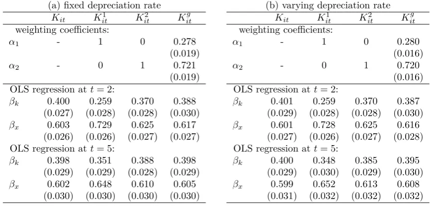
Table 3: Average estimates of weighting coefficients and technology parameters

(a) fixed depreciation rate

Kit Kit1 Kit2 K g it weighting coefficients:

α1 - 1 0 0.278

(0.019)

α2 - 0 1 0.721

(0.019)

OLS regression att= 2:

βk 0.400 0.259 0.370 0.388

(0.027) (0.028) (0.028) (0.030)

βx 0.603 0.729 0.625 0.617

(0.026) (0.026) (0.027) (0.027)

OLS regression att= 5:

βk 0.398 0.351 0.388 0.398

(0.029) (0.029) (0.028) (0.029)

βx 0.602 0.648 0.610 0.605

(0.030) (0.030) (0.030) (0.030)

(b) varying depreciation rate

Kit Kit1 Kit2 K g it weighting coefficients:

α1 - 1 0 0.280

(0.016)

α2 - 0 1 0.720

(0.016)

OLS regression att= 2:

βk 0.401 0.259 0.370 0.387

(0.029) (0.028) (0.028) (0.030)

βx 0.601 0.728 0.625 0.616

(0.027) (0.026) (0.027) (0.028)

OLS regression att= 5:

βk 0.400 0.348 0.385 0.395

(0.029) (0.030) (0.029) (0.030)

βx 0.599 0.652 0.613 0.608

(0.031) (0.032) (0.032) (0.032)

Note: The standard errors of Monte Carlo estimates are reported in parentheses.

should be more relevant for constructing the initial capital shock. The ex ante information on the DGP is in line with these estimation results, because X2 _{is the variable with the highest} correlation with the true capital. The bottom panels of Table 3 (a) and (b) summarize the cross-sectional estimations of technology parameters in (23) for two regression periods t = 2 and t= 5. The estimation results are stable with the fixed and varying depreciation rates. In the period following the initial capital approximation (t= 2), the approximation errors are not completely absorbed in the PIM. Thus, the estimates based onK1

it suffer from a downward bias as predicted in (10). This bias is less significant in the periodt= 5, but still persists. In both periods t= 2 and t = 5, the best estimates are those obtained when K2

it and K g

it are used as measures of capital. The estimation results forK2

itandK g

itare slightly improved in periodt= 5. The overall message of these Monte Carlo experiments is that the approximation error of the initial capital measurement affects the production function estimation, and the bias persists over time. In two cases this bias is negligible: i) when the initial capital is calculated based on a good proxy with a high correlation to the true values of capital (K2

it); ii) when the initial capital is calculated by using our generalized method that takes into account all available information (K_itg). The former is not feasible in many real-world situations because the correlation between proxy variables and the true initial capital is unknown.

5

Empirical application

In this section, we compare the performance of different initial capital approximation methods by using Luxembourgish firm-level data. The firm-level production data come from the Structural Business Survey (SBS) conducted by the statistical office of Luxembourg (STATEC). This is a yearly survey of firms registered in Luxembourg for years 2003 to 2011. Our data covers all industries represented in the Luxembourgish economy at the 2-digit level.5 _{The main variables}

of interest are: value-added output (Yit) deflated by the output price index; labour measured as hours worked (Lit); energy and intermediate material consumptions (Eit andMit, respectively). Capital stock is not directly observed, instead the data set provides total values of investments in tangible goods (e.g., equipment and buildings). The book value (BVit) of firm assets is available for years 2005 to 2011.

Similar to other firm-level data sets, our panel data are not balanced. Missing observations may be due to firms’ entry and exit, changes in the coverage of the survey, as well as due to the change in firms’ legal form, which are not always possible to track. Small enterprises with less than 50 employees or less than 7 million EUR turnover are sampled, other firms are all surveyed.6 _{In this data set, we do not observe the majority of firms over long time periods. Out}

of almost 4000 different firms in the data set, only 198 are observed for all periods of the sample. 75% of firms in our sample have at most 5 year-observations. Therefore, we should expect bias in production function estimation if initial capital stock is mismeasured.

5

The industry classification roughly corresponds to NACE.

6

For our empirical exercise, we select a subsample of the data by restricting it to only firms with at least 5 observations between 2005 and 2011. Time restriction is defined by the availability of the data on book value for firms in Luxembourgish SBS. There are 779 firms in this subsample, 277 of them are observed for every year.

5.1 Capital measurement

Within each industry group, we generate initial capital at the firm level using the shares of firms’ labour, energy, materials, and book value. We use the sum of book values of all firms within each industry as an approximation of the aggregate capital stock in 2005. The procedure is similar to the one in Monte-Carlo simulations: initial capital values are generated for the first year of the sample, i.e. 2005, then the PIM is applied to calculate capital for other years.

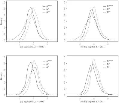
Figure2 (in Appendix) plots the distributions of different capital measures for the first and the last year of the sample. HereKbmel _{is generated according to the generalized method using} all available proxies, i.e. labour, material, energy, and book value; Kb _{is equal to book value for} the first period of observation; Ke _{is generated according to the share of energy consumption;}

Km _{and K}l _{are generated according to the share of material, and labour input respectively.} Capital stock measurements for every consecutive year are generated using the PIM. We also introduce book value (BV) as an alternative measure of capital. As the left panel of Figure 2

for year 2005 suggests, there is a significant difference in the distribution of capital according to different approaches (see also Table4). In Figure2(b) and (d) for year 2011, the distributions of capital measures are more similar due to adding deflated investment series to each initial capital measure, but still quite heterogeneous. Augmenting book value with investment data through the PIM increases the mean of the capital based on the book value in the first year (Kb_{) as} compared to simply using the book value (BV) as a measure of capital (see Figure3and Table

4). This increase is to be expected due to the common practice of accelerated depreciation that leads firms to understate their capital stocks.

Since we do not know the real value of the capital stock in this sample, we cannot say which proxy is the best. However, the weights calculated using generalized method favour the share of materials as the best proxy, followed by book value (see Table 5 in the next subsection).

5.2 Production function estimation

Similar to Monte Carlo experiments in the Section 4, we compare different approximation meth-ods in the context of production function estimation. Consider value-added Coob-Douglas pro-duction function with capital and labour as input variables. The corresponding parameters are denoted byβkandβl. Unlike in the Monte Carlo study, we estimate the two technology parame-ters by using the control function approach (Olley and Pakes,1996), because input variables are likely to be correlated with error terms due to unobserved productivity shocks.7 _{The production}

7

Table 4: Descriptive statistics of different approximations of capital, balanced sample

logBV logKl _logKe _logKm _logKb _logKbmel

t=2005

Min. 6.683 11.89 7.056 10.78 6.701 9.949

1st Qu. 12.354 14.71 13.882 14.32 12.286 13.114

Median 13.881 15.59 15.134 15.26 13.784 14.124

Mean 13.661 15.71 15.052 15.39 13.592 14.203

3rd Qu. 15.098 16.61 16.243 16.4 15.003 15.238

Max. 20.68 21.96 21.778 21.72 20.568 20.681

t=2011

Min. 3.418 10.57 10.69 11.38 8.652 10.5

1st Qu. 11.814 14.56 14.02 14.07 12.589 13.2

Median 13.491 15.38 14.99 15.12 14.06 14.3

Mean 13.347 15.58 15.14 15.24 13.994 14.42

3rd Qu. 14.919 16.53 16.13 16.2 15.303 15.46

Max. 20.318 21.82 21.34 21.33 20.362 20.31

function estimation results based on different capital measurements are reported in Table 5.

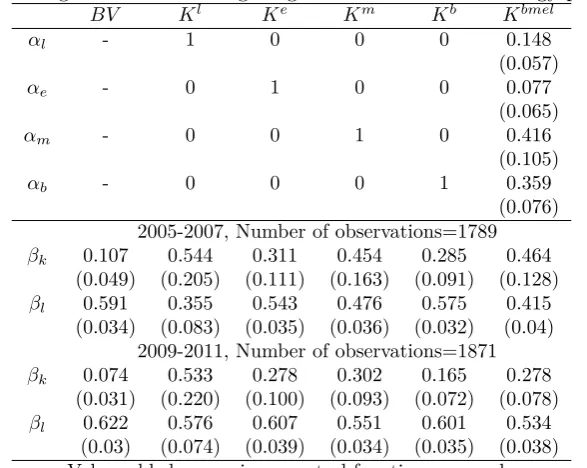
Table 5: Average estimates of weighting coefficients and technology parameters

BV Kl _Ke _Km _Kb _Kbmel

αl - 1 0 0 0 0.148

(0.057)

αe - 0 1 0 0 0.077

(0.065)

αm - 0 0 1 0 0.416

(0.105)

αb - 0 0 0 1 0.359

(0.076) 2005-2007, Number of observations=1789

βk 0.107 0.544 0.311 0.454 0.285 0.464

(0.049) (0.205) (0.111) (0.163) (0.091) (0.128)

βl 0.591 0.355 0.543 0.476 0.575 0.415

(0.034) (0.083) (0.035) (0.036) (0.032) (0.04)

2009-2011, Number of observations=1871

βk 0.074 0.533 0.278 0.302 0.165 0.278

(0.031) (0.220) (0.100) (0.093) (0.072) (0.078)

βl 0.622 0.576 0.607 0.551 0.601 0.534

(0.03) (0.074) (0.039) (0.034) (0.035) (0.038)

Value added regressions, control function approach, industry dummies included.

The upper panel of Table 5 summarizes the assumptions and/or estimates of weighting coefficients. The lower panel provides the Olley-Pakes estimation of technology parameters for the first and the last three years of the sample.8 _{All coefficient estimates are significantly}

different from zero. Similar to the Monte Carlo evidence, the estimates of βk are significantly

8

different for Km_,Ke_,Kb _andKl_{, however, there is no reason to prefer one estimate over others.} The lowest estimates are obtained in the case of BV and Kb_.

The generalized method values the material variable as the most relevant proxy assigning the weight of 0.42 to it, the second most relevant proxy is the book value, which is attributed 0.36 of correlation to true capital. Based onKbmel_{, we obtain capital coefficients of 0.464 and 0.278,} respectively for the first and the last three years of our sample. The results for the last three years of the sample are more homogenous due to a stronger impact of the PIM on the capital measures with the exception ofBV, on which the PIM was not applied. However, note that the coefficient on Kl _{is biased in both periods implying that the initial error in the measurement of} capital still persists after several periods.

6

Conclusion

In this paper we address the problem of the initial capital generation, which is especially relevant for the data sets with short time horizon due to severe bias caused by errors in the measurement of capital. We present a new estimation method to deal with the problem of missing capital for the purposes of production analysis. This method generalizes the existing methods of initial capital approximation. Instead of arbitrarily choosing a proxy for distributing the aggregate capital among firms, we introduce a stochastic multivariate function of proxies according to which the capital is allocated. We estimate the weights of the proxies using the inverse PIM and therefore do not rely on an arbitrary choice of a proxy. These weights reflect indirectly the correlation between proxy and capital, therefore capturing the quality of proxies.

We conduct a series of Monte Carlo experiments to test the performance of the new method and compare it with the common ad hoc approaches. The traditional methods that we tested rely on a single proxy and assume deterministic relationship between this proxy and capital. In contrast, the generalized method uses multiple proxies. It performs as good as the single-proxy approach applied to the best proxy. Since when working with real data one does not know which variable is the best proxy, the generalized method is a very promising tool for initial capital generation.

There are several directions in which the proposed method can be further improved in the future. The generalized method is based on a set of assumptions which allow us to focus on the initial capital problem. Although these assumptions are standard in the literature, some of them could be relaxed depending on the availability of empirical data or preliminary knowledge of the patterns of capital accumulation. For example, the PIM can be modified to include the capital asset retirement (OECD,2009), a country-specific depreciation rate (Schündeln,2013), and to relax the assumption that productive capital services are proportional to capital stock (Müller,

Appendix

0 1 2 3 4 5

0. 0 0. 2 0. 4 0. 6 0. 8 1. 0 D en si ty True value K1

0 1 2 3 4 5

0. 0 0. 2 0. 4 0. 6 0. 8 1. 0

(a) log capital,t_{= 1} True value

K2

0 1 2 3 4 5

0. 0 0. 2 0. 4 0. 6 0. 8 1. 0 True value Kg

0 1 2 3 4 5

0. 0 0. 2 0. 4 0. 6 0. 8 1. 0 D en si ty True value K1

0 1 2 3 4 5

0. 0 0. 2 0. 4 0. 6 0. 8 1. 0

(b) log capital,t_{= 5} True value

K2

0 1 2 3 4 5

0. 0 0. 2 0. 4 0. 6 0. 8 1. 0 True value Kg

Figure 1: Distributions of capital measurements in the Monte Carlo experiment.

10 15 20 0. 00 0. 05 0. 10 0. 15 0. 20 0. 25 0. 30

(a) log capital,t_{= 2005}

D en si ty Kbmel Kb Km

10 15 20

0. 00 0. 05 0. 10 0. 15 0. 20 0. 25 0. 30

(b) log capital,t_{= 2011}

Kbmel

Kb

Km

10 15 20

0. 00 0. 05 0. 10 0. 15 0. 20 0. 25 0. 30

(c) log capital,t= 2005

D en si ty Kbmel Ke Kl

10 15 20

0. 00 0. 05 0. 10 0. 15 0. 20 0. 25 0. 30

(d) log capital,t= 2011

Kbmel

Ke

Kl

Figure 2: Distributions of capital measurements, traditional and generalized approaches.

5 10 15 20

0. 00 0. 05 0. 10 0. 15 0. 20 0. 25 0. 30 D en si ty Book value Kb

References

Atkinson, M. and Mairesse, J. (1978). Length of life of equipment in French manufacturing industries. Annales de l’insee, (30-31):23–48.

Becker, R. A. and Haltiwanger, J. (2006). Micro and macro data integration: The case of capital. In A New Architecture for the U.S. National Accounts, NBER Chapters, pages 541– 610. National Bureau of Economic Research, Inc.

Berndt, E. R. and Fuss, M. A. (1986). Productivity measurement with adjustments for variations in capacity utilization and other forms of temporary equilibrium. Journal of Econometrics, 33(1-2):7–29.

Diewert, W. E. (1980). Aggregation problems in the measurement of capital. InThe Measure-ment of Capital, NBER Chapters, pages 433–538. National Bureau of Economic Research, Inc.

Fisher, F. M. (1965). Embodied technical change and the existence of an aggregate capital stock. The Review of Economic Studies, 32(4):263–288.

Foster, L., Grim, C., and Haltiwanger, J. (2013). Reallocation in the great recession: Cleansing or not? Working Papers 13-42, Center for Economic Studies, U.S. Census Bureau.

Gilhooly, B. (2009). Firm-level estimates of capital stock and productivity. Economic and Labour Market Review, 3(5):36–41.

Hall, B. H. and Mairesse, J. (1995). Exploring the relationship between R&D and productivity in French manufacturing firms. Journal of Econometrics, 65(1):263–293.

Hicks, J. R. (1974). Capital controversies: Ancient and modern. American Economic Review, 64(2):307–316.

Hulten, C. R. (1991). The measurement of capital. In Fifty Years of Economic Measurement: The Jubilee of the Conference on Research in Income and Wealth, NBER Chapters, pages 119–158. National Bureau of Economic Research, Inc.

Jorgenson, D. W. (1963). Capital theory and investment behavior. The American Economic

Review, 53(2):247–259.

Leontief, W. (1947). Introduction to a theory of the internal structure of functional relationships. Econometrica, 15(4):361–373.

Levinsohn, J. and Petrin, A. (2003). Estimating production functions using inputs to control for unobservables. Review of Economic Studies, 70(2):317–341.

Martin, R. (2002). Building the capital stock. Working paper, The Centre for Research into Business Activity (CeRiBA).

Müller, S. (2008). Capital stock approximation using firm level panel data. Discussion Paper 38, Bavarian Graduate Program in Economics (BGPE).

OECD (2009). Measuring capital. OECD, Paris, France.

Olley, G. S. and Pakes, A. (1996). The dynamics of productivity in the telecommunications equipment industry. Econometrica, 64(6):1263–1297.

Pakes, A. and Griliches, Z. (1984). Estimating distributed lags in short panels with an application to the specification of depreciation patterns and capital stock constructs. Review of Economic Studies, 51(2):243–262.

Pavcnik, N. (2002). Trade liberalization, exit, and productivity improvement: Evidence from Chilean plants. Review of Economic Studies, 69(1):245–276.

Raknerud, A., Rønningen, D., and Skjerpen, T. (2007). A method for improved capital mea-surement by combining accounts and firm investment data. Review of Income and Wealth, 53(3):397–421.

Schündeln, M. (2013). Appreciating depreciation: Physical capital depreciation in a developing country. Empirical Economics, 44(3):1277–1290.

Solow, R. M. et al. (1960). Investment and technical progress. Mathematical Methods in the Social Sciences, 1:48–93.

Stevens, G. V. (1989). A substitute for the capital stock variable in investment functions. Inter-national Finance Discussion Papers 386, Board of Governors of the Federal Reserve System.

Swamy, P. A. V. B. (1970). Efficient inference in a random coefficient regression model. Econo-metrica, 38(2):311–323.