An Analysis of Errors in the Electric Analog Computer

AN ANALYSIS OF ERRORS

IN THE ELECTRIC-ANALOG COMPlYrER

Thesis by

William Joseph Dixon

In Partial Fulfillment of the Requirements for the Degree of

Doctor of Philosophy

California Institute of Technology Pasadena, California

The author wishes to express his indebtedness to those whose work and interest have made this thesis possible.

Thanks are due Dr. G. D. McCann for having made the California Institute computer available for the purpose of conducting these investigat ions; to Dr. R. H. MacNeal, whose helpful suggestions have led the way to many of the theoretical developments; and to Dr. C. H. Wilts for the contribution of corroborating experi-menta 1 evidence.

ABSTRACT

This thesis is the result of work done in connection with the California Institute of Technology

Electric-Analog Computer. Several methods are developed for

determining the accuracy of the solutions of various types of problems by electric circuit analogies. These are

used to obtain expressions for the errors involved in the solutions of specific examples.

The first part deals with the error involved in the solution of problems with continuously distributed physical properties by means of circuit analogies of lumped para-meters. The errors of mode frequencies of several mechan-ical vibration problems are given in the form of asymptotic ser:i.es.

In thB second part, investigation :Ls made of the effect of the statistical deviation of the actual values of the computer elements from their nominal values. This effect is computed for circuits for some of the problems con-sidered i n the first section.

PART

I

I I

III

TITLE PREFACE

ERRORS DUE TO

T

H

E

LUMPING OF CONTINUOUS PHYSICAL PROPERTIES

1.1 Introduction 4

1.2 The B'ourth Order Eigenvalue Problem 5 1.3 Solution by Wave Propagation

Characteristics. Simply Supported Beam.

1.4 Solution by Asymptotic Series.

11

Cantilever Beam. 13

1.5 The Second Order Eigenvalue Problem 27

1.6 Unequal Lumping 30

THE EFFECT OF STA'rISTICAL DEVIA'rION OF THE VALUES OF '11

HE ELEMENTS

2.1 General 35

2.2 The Second Order Eigenvalue Problem 39 2.3 The Fourth Order Eigenvalue Problem 41 2.4 Distribution of the Elements of the

California Institute Computer 43 LAJ\JDING TEST OF A MODEL AIRPLA1TE WING

3.1 Experimental Test 48

3.2 Analytical Methods of Computation 49 3.3 Analog Computer Solution 51 References

List of Appendixes List of Symbols

PAGE 1

4

35

48

1

PREFACE

The statement of a problem which is to be solved with the electric-analog computer consists of three distinct parts. The first part is a description of the system. This may be in the form of a set of mathematical equations, or i t may be a description of the subject of the problem, consisting of physical measurements and properties. The second part establishes the excitation of the system. The third part states what answers are desired; that is, prescribes the quantities to be in-vestigated.

The solution of the problem follows the same steps. First an electric circuit is constructed which is an ana-log of the physical or mathematical system. The second step is the application of electrical excitati on to various parts of the circuit. And finally the answers are obtained by observation of the electrical ~uantities present in

the circuit.

Errors in the solution may be traced back to one of these three processes. The analogy between the electric circuit and the physical or mathematical system may be faulty. The excitation of the electric circuit may not

imperfect analogy.

The other sources do contribute to errors, and in many classes of problems cannot be ignored. When the

excitation consists of an arbitrary function of time to be applied to the circuit, the combatting of error from this source lies chiefly i n the design and use of special equipment to generate the desired functions. ( 1 ) I \ .. Errors due to metering may be caused by the disturbing of the analog-circuit when the meters are connected, or by transmitting to the operator information at variance with that which exists in the circuit . The elimination of these errors lies in metering-system design, in which the chief limitations are the qual i ty of ferromagnet ic materials and parasi t ic impedances.

The analogy between the physical or mathematical system and its elecbric analog may be inaccurate for a number of reasons. One is that the di fferential equations of the original system may be represented i n the circuit by difference equat ions. This i s most often the result of using lumped electrical parameters as an analog of distributed physical properties which are functions of a continuous space variable. Errors belonging t o this class are considered in Part I of this thesis.

Another reason is the imperfection of the individual

3

elements of the computer, including inherent parasitic inductance, capacitance, and resistance; deviation of the actual value from the nominal value; and non-lineari t ies in the operating characteristics. Part II deals with the limitation of precision caused by the deviation of actual

values from nominal values.

A third reason is that it may be impossible to

reduce the original physical system to a set of equations without introducing several qualifying assumptions which affect the validity of the answers obtained.

In discussing the error and precision involved in the solution of a problem by means of a certain circuit i t is necessary to specify what quantity constitutes the answer in order to define the error and precision. It would be o2fficult to define and ascertain the error of an answer which consists, for example, of the response

of a system to an arbitrary transient excitation. In the case of vibration problems, the frequency of normal

I ERRORS DUE TO THE LUMPING OF CONTINUOUS PHYSICAL PROPERTIES

1.1 Introduction

The theory underlying the construction of

elec-tric circuits of discrete elements to represent continuous

physical systems has been considerably developed. (2 ,3)

The most certain method of determining the error

intro-duced by the lumping of parameters is to calculate the

solution to the physical problem, calculate the solution

of the circuit analogy, and compare the results. This

cannot be done in general, for the usual problem to which

the computer is applied cannot be solved by exact

analyt-ical methods. However the process of checking any com

-puter involves using i t to get answers to problems whj_ch

can be solved by other means. It is then hoped that the

errors present in the general solutions can be estimated

from a knowledge of the errors which exist in the test

problems.

Certain eigenvalue problems are a good test for

errors introduced by lumping parameters, for solutions

may be obtained for the problem with continuous

proper-ties, as well as for the electric circuit which

repre-sents it. The electrical analogy for this type of problem

is a passive, non-dissipative circuit, for which the

nor-mal modes of oscillation are determined. For the purpose

5

be the answer.*

In th is pa rt are considered eigenvalue problems associated with linear second and fourth order partial differential equations wit h constant coefficients. For the continuous physical system the eigenvalue solution is obtained from a differential equation by standard methods. For the lumped circuit the mode frequencies are obtained from t he solution of a difference equation or difference equations. For many of the cases considered the mode frequencies cannot be expressed explicitly from the difference equation solution, but are developed from i t i n the form of series.

1.2 The Fourth Order Eigenvalue Problem

The eqt~tion considered here is that describing the lateral motion of a uniform beam bending in one plane.

0

₄

_~

'°

_aa.

o

x

+ EI

8

t~

= O

y lateral deflection x - longitudinal dimension

p

= mass per unit length

EI = stiffness to bending in x-y plane t = time

Effects of rotary inertia, finite shearing strain, * If the physical system under consideration is

non-conservative, but has linear dissipation, the same method may be used. The circuit will contain resistance, and

the mode frequencies wil l be complex numbers, represent-ing rate of decay as well as rate of oscillation.

and damping are neglected. To reduce this to an eigenvalue

problem* sinusoidal oscillati ons are assumed to exist at

a frequency of

w

/2

rr

.

y(x,t) is replaced by Y(x)ej~t, and

o

2

_y

is replaced by -oo

2

Yejwt. Equation

(1)

is now written

a

t

2

~

~;

- k 4 y = 0' ( 2 )

(p

wi)'.-:

where k == - 4•

EI

k

is a positive, real number. In general

Y

is a complex

number. However, in normal mode vibrations, all portions of

the sys tern vibrate in the same phase, so that Y may be

considered real without loss of generality. y is determined

"<.t>t

by taking the real part of

Y

eJ • The general solution of

equati on (2) is

Y

=

A cosh kx + B sinh kx

+

C cos kx + D sin kx. (3)

For comparison with solutions by finite-difference

methods, two sets of boundary conditions are applied,

giving the following standard solutions. (4 )

(a) Simply supported beam.

At x - 0, Y

=

0 and d2Y

o.

dxz -d2y

At x -:::: 1 , Y = 0 a nd _ O • dx2.

km= m 'Tt

( 4)

( 5)

7

m

=

1, 2, 3, •.. (b) Cantilever beam.

At

x - 0, Y

=

0 and -dY = 0.

d2Y dxd3Y

- 1,

dX.Z'

= 0 and

dX3

= O.

(Clamped end. )

At

x

(Free end. )

Y : ~(cosh kmx - cos kmx)

+

Bro

(

s i nh kmx - sin kmx ) , ( 6) where km is a solution of the equation

1 + cosh k cos k :

O,

(7)

and

§ii

-Am - _sinh cosh km_km +

₊

cos _{sin km} km = (-l)m(tan

~km

l

_~

(-l)

m

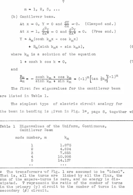
The first fevv e·igenvalues for the cantilever beam are listed in Table 1.

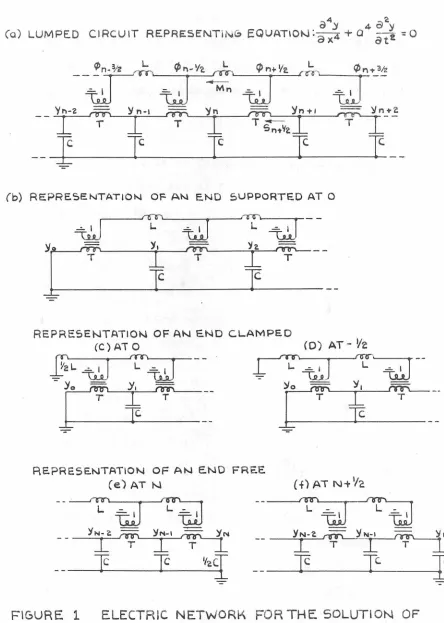
The simplest type of electric circuit anal ogy for

the beam in bending is given in Fig. l*, page 8, together with

Table 1 Eigenvalues of the Uniform, Continuous, Cantilever Beam

mode number, m km

1 1.875

2 4.694

3 7.855

4 10.996

5 14.137

[image:11.614.126.557.54.688.2]

a'°'y

4 a~

(o) LUMPED Cl RCU IT REPRESENTiN(.;

EQUATIO~:

a

4

+

Q

~

= 0

x

at

q,n-o/z L.

-~ '--~---1.Mn ¢ n-'h

L

'Pn+l/e

~~

..

_3~

w

yr.-?. Yn+1 '!Jn+?.

T - T

5 n..'fi

__ f

r

I

I

__

(b) REPRESENTATION OF A"1 E.ND 5UPPORTE.D AT 0

L.

~--1

f"ll"T\

y,

f"ln"'I - 'Y 2. ' T l r \ - - -

-T

t

T

f

T

-REPRESENTATIO~ OF AN E.ND C.LAMPED (C) Ai 0

ri:

ffrl

tfL~J

L

~

e

i

Cf'---REPRE.SE.NTATION OF At-J E.ND FREE

[image:12.612.118.562.67.690.2]

(e)AT t--1 (~)ATN+1/c

FIGURE

1

ELECTRIC NETWORK

FOR THE

SOLUTION

OF

9

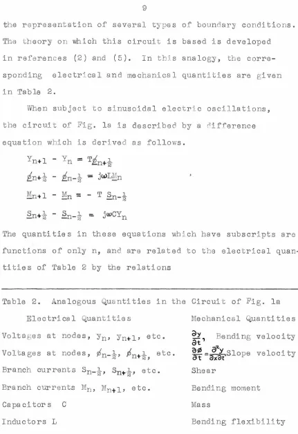
the r epresentation of several types of boundary conditions. The theory on which this circuit is based is developed

in references (2) and (5). In this analogy, the corre-spending electrical and mechanical quanti t ies are given

in Table 2.

When subject to sinusoidal electri c oscillations,

the circuit of Fig. la is described by a c'ifference

equation which i s derived as follows.

,,/ n +.±.

E.. 2

Mn+l -

Mn

=

-

T Sn-!

The quantities in these equations which have subscripts are

functions of only n, and are related to the electrical quan-tities of Table 2 by the relations

Table 2. Analogous Quantities in the Circuit of Fig. la Electrical Quanti t ies

Voltages at nodes, Yn, Yn+l ' etc. Voltages at nodes, ¢n-!' Pn+!, etc.

Branch currents Sn-!, Sn+! ' etc. Branch currents Mn, Mn+l ' etc.

Ca pa ci tors C Inductors L

Mechanical Quantities

~Y Bending velocity

at'

0¢ = a-z.y Slope velocity

di

a.xe>t'

Shear

Bending moment

Mass

[image:13.612.123.554.48.676.2]

10

Yn(t)

=

(R(Yn ejoot )

¢n+t (t) =

(R

(tn

+

i

ejwt ) Mn(t)

=

(R (Mn ejwt)

Sn

+

i

(

t)

=

CR

(.§n+!

e

jwt).

<Rmeans "the real part of. 11 _{The four dif:'erence equations}

may be reduced to one by substituting for the terms on the

left side of each equation according to the preceding

equation. 'rlie result of this process is

Yn+2 - 4yn+l + (G-z4 ) yn - 4Yn-l + Yn-2

=

O where

z

=

'./

T

w

{LC

,

and is real and positive. The general solution of this difference equation is

( 8)

Yn

=

A co sh nel

+

B sinh n81 + C cos n82

+

_{D sin ne 2} (9) in which ₉₁ and _{82 are} d etermj_ned from the equation

2 sinh ₂₈₁ l = 2 sin 282 l = z

₌

_y

_T

_w

_M

_.

(10) The details of this solution are given in Appendix 1.

Equations (8) and (9) are ~alid for 2 ~ n

<

N - 2 when the end conditions aro those given i n Figs. lb to lf.

By

writing out the equations of these terminating circuits and defining Yn for n

<

:G and N - 2

<

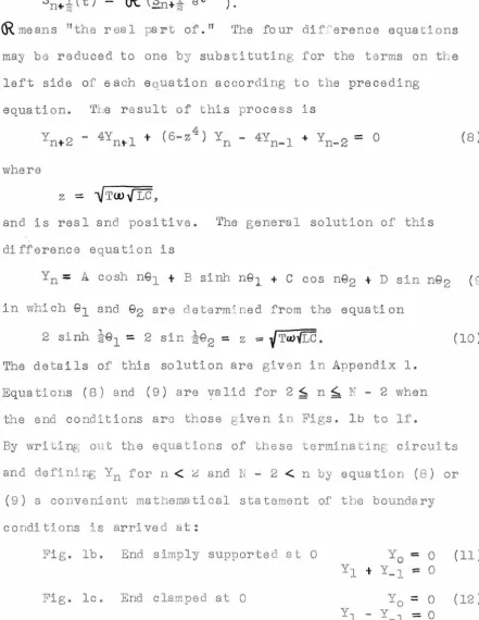
n by equation (8 ) or

(9) a convenient mathematical statement of t he boundary conditions is arrived at:

Fig. lb. End simply supported at 0 _Yo = 0 (11)

Y1 t y_l :::: ₀

[image:14.615.124.565.161.731.2]

11

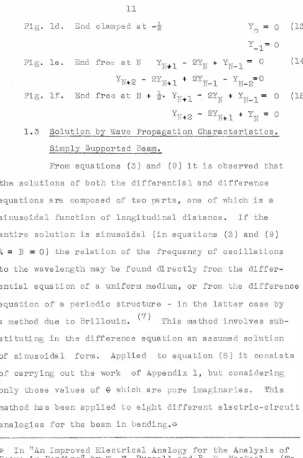
Fig. ld. End clamped at -2 l yo = 0 (13)

y _{= 0} -1

Fig. le. End free at N _YN+l

-

_2YN + _YN-1

=

0 (14)

YN+2

-

2YN+l + 2YN-l

-

YN-2=0

i:;i· _{lf. End free at N +} l

YN-t-1

-

2YN + YN-1

=

0 ( 15)

,ig. 2·

1.3 Solution by Wave Propagation Characteristics. Simply Supported Beam.

From equations (3) and (9 ) i t is observed that the solutions of both the differential and di fference equations are composed of two parts, one of whi ch is a sinusoidal function of longitudinal distance. If the entire solution is sinusoidal (in equations (3 ) and (9) A = B

=

0) the relation of the frequency of oscillations

to the wavelength may be found directl y from the differ-ential equation of a uniform medium, or from the difference equation of a periodic structure - in the latter case by a method due to Brillouin. (? ) This method involves sub-stituting in the difference equation an assumed solution of sinusoidal form. Applied to equation (8) it consists of carrying out the work of Appendix 1, but considering only those values of

e

which are pure imaginaries. This method has been applied to eight dLfferent electric-circuit analogies for the beam in bending.*

[image:15.612.126.554.48.695.2]

12

Referring to the differential equation (2), and its

solution, equation (3), and setting 'A = B

=

O, wavelength

A

and oscillatory frequency are related as follows.

21t = 1< ::::

(fW2)~

>.

-

EI

Similarly, from the difference equation (8) and its

solution, equat ion (9), result s the r elation

8₂ :::::: 2 s i n-1

iz

= 2 sin-' [

i (

T 2 w 2 LC )

~]

•

( 16)

( 17)

e

₂ is the finite-difference equivalent of k, the wave number.

From equation (4), the simply supported, conti nuous

beam has sinusoidal mode shapes. The equivalent circuit

of N cells analogous to this wi l l bave the end condition

of Fig. lb at nodes 0 and N. It is apparent from equations

(11) that the end conditions wi l l be satisfied by a

sinus-oidal solution:

Y = A sin mn1l

n

N

m ;:: 1, 2, 3, ••• , N - 1

so that the frequency may be obtained from

3 Z ; 2 sin -1.g - 2 sin mit - 2 sin km km k""

"' - 2 z - 2N - - 2N

=

N - 24N3

k 5

+

lg2o

N

s

-

...

Except for an over-all factor relating time measurements

i n the analogous systems, the circuit is constructed to

satisfy t he equati on

N4T2LC - p

- EI

This allows comparison of the mode frequencies of the

two systems

,6w,... CJJm _ 1 - Zm2 •

-../P

-

1

~ = CVrno -

T

=I/

LC

""

k

.,.

~

1/

E

r'

- 1

(18)

(19)

13

sin2 km

.6.lRJ"' == 2N

-

1

Wmo

_{

_k

_mt

2N

AW"' km 2

k

m

4

+

-

.

.

.

( 21)

- -_Wmo = _{- 12N}20 _360N4

km

-

m1t ( 5)

As in the case of the clamped and free ends

illus-trated in Fig. 1, an analogy can be constructed for a

support midway between nodes. 'rhe equations for this type

of analogy are satisfied by a sinusoidal mode shape. Thus

the preceding development is applicable, and equation (21)

gives the correct error, provided N represents the

effec-tive length in cells.

1.4 Solution by Asymptotic Series. Cantilever Beam.

Unless the boundary conditions permi t a

sinus-oidal solution the method of wave propagation characteristics

cannot be used to determine the mode frequencies. For the

uniform beam, only t he beam with both ends simply supported

will have a sinusoidal mode sbape. Problems involving

other end conditions must be attacked by different methods.

'l'he cantilever beam is an important object of study on

the electric analog computer. A method of analysis

suggested by R. H. MacN~al is employed here to determine

the error in mode frequencies of circuit-analogies of the

cantilever beam based on Fig. 1, and to compare i t with

the error in mode frequencies of the simply supported

beam of the preceding section.

given in Fig. 1. These will be designated (ce), (cf),

(de), (df), the (ce) beam having the end condition of Figs.

le and le, etc. 'rhese are summarized in Table 3, page 15.

The first step is to reduce the general solution to the difference equation,

Yn = A co sh n81

+

B sinh ng1 + C cos n82 + D sin n82 , (9) and the boundary conditions to a form analogous to equation

(7) of the continuous beam. This is essentially a process

of browbeating hyperbolic and trigonometric functions.

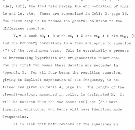
For the first two beams these details are recorded in Appendix 2. For all four beams the resulting equation, giving an implicit expression of t he frequency, is

ob-tained and given in Table 4, page 16. The length of the circuit-analogy, measured i n cells, is designated M. It will be noticed that the two beams (cf) and (de) have

identical equations, and hence will have identical mode

frequencies.

It is seen that both members of the equations in

Table 4 are functions of z, and hence of W . The solutions

could be found by plotting these functions on a graph and

noting the points at which the functions are equal. This

method is of limited value as it would tave to be repeated

for each value of M.

The equations of Table 4 may be put in a form which

[image:18.615.113.563.87.520.2]

Table 3 Sum m ary of Cantilever Be ams Considered Bea m Cla mp ed F'ree M , Length Boundary Designation at at in Cells Conditions ( ce) 0

N

N

Y o= 0 Y a -Y -1 = 0 Y N+l

-2 Y N

-+

y N-l == 0 Y N+4 -2Y N+I

+

2Y N -I -Y = O N-2. (c f) 0

N

+

i

N

+

1=. 2

Table 4 Implicit Solution of F'inite-Difference Can t ilever Beam M ode Frequencies 2 sinh ie , = 2 sin ie 2 ~ z = {T(.IJ-{Lc

Beam (

ce) 1

+

cosh Me 1

1

+

c osh

M

e

1 (cf) }

and (de

) Implicit Solution cos M e2

=

sinh

M

e

1 sin -sinh M e , sin cos M G 2 = 1 -h l · cos 28 1 = 1 -

v1

-~

;

M

e

2 tanh ~ -e , tan .,,-z Z M 92 --~·

Vi=

z4

4

-

16 cos ie 2 ie , ( df) 1

+

cosh M9 1 cos M e2 sinh

M

e

,

sin M9 z tanh ie , tan is 2 -sinh M Q 1 sin

M

e

2 continuous 1

+

cosh k cos k ~ 0 beam z

2.

4

ij

17

and not restricted to discrete values. Now, as the expansion desired wi l l be for large values of M, replace

l

M by w-2. Also, for convenience, replace z by v ,/W. By these means , any of the equat ions of Table 4 may be put in

the form

f

·

=·

f ( v' w)

=

0. ( 22)

Furthermore, each of these is satisfied by

f ( k m, 0 ) = 0 , ( 2 3 )

in which

k

m

is any solution of equation

(

7).

It is assumed that a solution exists of the form v = v(w).

D e Sl . gna ing t·

av

a

and

~

by subscripts v and w, respectively, 2

a n:1 dv and d

v

dw dwz by v' and v", respectivel y, successive

differentiation of equation (22 ) with respect tow results

in

df : fvv' + fw- O dw

These equations may be solved for v 1 ,

v

'

-

_ f w

f v

f v12

VII - - _{""'f_v} >IV _{_ _}

2

f vv fw + fv 3

=

-2fvwV1 _fww

- fv -

r;--2fvw fw fww fvZ

:r;-Then the function v(w) may

_.

be written wv' w2 "

~ - - + v + •••

l!

2 l

v"

'

etc.

v', v", etc., are to be calculated from equations (27),

(28), etc., in which the partial derivatives o f f are all ( 24)

(25)

( 26)

( 27)

evaluated at (km,O). According to the theory of implicit

functions (8 ), this development of v(w) is valid provided

f

v (km

P)

is different from zero, and f and all its

deriva-tives used in equations (26), (27), etc. exist and are continuous in the neighborhood of

(k

m

,O).

For example, applying the transformations stated at the

beginning of the preceding paragraph to the second equation of Table 4 results in

f(v,w)·=.·cosh (J sinh' v't:) cos (Jw sin-1 v;w)

( 29)

It is necessary to restrict this definition of f to values

of w other than zero. Wben w

=

0,

f(v,w)

=

f(v,O)·=· cash v cos v

+

1 (30) It is not immedi ately apparent that this function satisfies

the provisions stated at the end of the precedi ng paragraph, but they may be verified by recourse to the fundamental

definition of partial differentiation, or by expansion of the expressions in parentheses in equation (29) in power

series in (v w). (The existence of such series is of

interest, as i t shows that the partial derivatives in

equa-tions (26 ) and (27) will exist; that v may be expanded in

powers of w, and hence in the even powers of 1. and that

- M'

z may be expanded i n odd powers of 1 )

M"

The solution of a problem by the method of implicit

functions will be given later, in Appendix 4, in wLich a problem from section 1.6 is solved. The present problem,

frequen-19

cies, is obtained by a somewhat different, but related method, as follows.

From the above development, and by comparison with the simply supported beam, i t is expected that the

difference between Mzmand km, defined as

Mz-k

- k - '

U

·=·

( 31)

will hBve an expansion of the type

u

=

_IVIa2 , + ~ _M4 + •• • ( 32)

so that

z =- k (l+u )= k (1 + §.• + 8_{2+••• )}

M M Ma Mq • (33)

(Subscripts m, designating mode number, are understood.)

The equations of Table 4 are attacked by substituting appro-1

priate double power seri es in u and M~for the terms z, 91 ,

9z, etc. The amount of calculation is kept within reason

by maintaining a balance among the various orders of

infini-tesimals consistent with the number of terms a, , a₂ , etc., desired. The zero order terms always cancel by virtue of equation ( 7 ) •

infinitesimals.

T erms in u, . -1 a

M constitute the first order

Terms in u2 , ul/I~ 1 constitute the second

I ~ M4

order infinitesimals, and so forth. This calculation is carried out for the (ce ) beam in Appendix 3, wi th the first two terms in the expression of error determined.

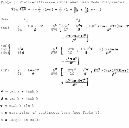
The results for all the cantilever beams considered

are given symbolically in Table 5, page 20, and numerically

in Table 6, page 21. Figs. 2 and 3, pages 22 and 23,

Table 5 Finite-Difference Cantilever Beam Mode Frequencies

i/

T

wv

LC = z =

~

( l+u) =

~

( 1 +

~

~

+

~

!

+ , .. )

Beam

( c e ) _{- 24} k

and (cf)} k2a.

(de ) - 24(3

(df ) k • k<X.+67

- 24 {3

o. = tan k

+

tanh k

(3

=

tan k - tanh k

~

=

sinh k sin k

a2

[33k 2

- k 3

'l'

+

10

/3

k 'Y(ka.-6 'Y)2]

+

133

( 2k2 ~ 9ka.-12.)') ( koc-6'Y)

(JZ

k 3

r _

27k

+

18-k2'Y

+

k ( 2k+3cx.)a:

576

L

lo

ra

₁₃

2

k:z

?"<Y..ZJ

+

~3

k2. [ - 87k2 - k3

?'

+

(

2k

~

-3ka.+12l')(k'1+6?')

576 10

f3

ts"'

'

+

k?'(ka.+6'Y

yz.]

t33

k

=

eigenvalue of continuous beam (see Table 1)

[image:24.617.126.573.48.493.2]

21

Table 6 F'ini te-Difference Cantilever Beam Mode Frequencies

Beam

( ce ) ( ce )

(cf)} and

(de)

( df) ( df)

Z = k _M ( 1 + a_~n, _. + _-a~ _{4+ ···}) _.

_.1 M

Mode _al

1 -.423

2 -2.15

1 -.0789

2 -.952

1 • 26 5

2 .243

a2 b1 b2

.224 -.846 .628

8.64 -4.35 21. 9 - • 0757 -.158 -.145

.359 -1. 90 1.62 .0254 • 530 .121 -2.35 .486 -4.64

Table 7 Limiting Values of the Terms Giving the

Higher Mode Frequencies of Finite-Difference Cantilever Beams

Beam _{al a2}

( ce) k (k+6) k2 (k2+100k+240)

24 1920

(cf)} _{k2. k4}

and

(de) - 24 192o"

(df) k(k-6) k2 (k2 -100k+240)

[image:25.612.116.537.49.532.2]

·-tt :tt

m

~:JJ:r-t

-m

11!i

m

:

++

-

-~ ++ H -h ~TTI- =-,":t-J:

· r m · '::er .-· ' c'-1- -i-H-~J+J

- _{l-H--i-+++-'-+++l-t--H}-r-_{H_-++µ}~ _{_•__J·}• _{H_~}--_·-1-1":t ,:[-r -'+-'-+ _-1::'.:q:

beam mode frequencies and experimental errors determined

by C. H. Wilts, for the first and second modes, respectively. 'rhe experimental data of Fig. 3 vvere obtained at a computer frequency higher than optimum, at which the effect of

parasitic capacitance and inductance was appreciable. Consequently points vvere 8lso obtained in which a correction was made to account for this effect.

A comparison of the error of mode frequencies of the

cantilever beam with that of the simply supported beam is

made by comparing the coefficients of (k/~.02 in the

expansions of either u or (Aw/ wo). The coefficients of (k/M )2 rather than of ( l /M )2 are c onside red be cause the former gives the error in terms of the number of cells

per wavelength of the sinusoidal part of the solution. On this basis, i t is found that, for the first mode, only

the (cf) and (de) cantilever beams have less error than the

simply supported beam, and for the second mode, only the (df) cantilever beam has less error than the simply

supported beam.

In the higher bending modes of the uniform cantilever beam, the sinusoidal part of the solution predominates in

25

remaining terms become insignificant by comparison. Specifically

13-• ---

(-l)m 2 e-k

ex.

/3

---?'

f3 - - -I

In this manner, the limiting values of a, and a₂ are

determined. These are given in Table 7, page 21. Because

of the exponential nature of the terms involved, the convergence to these forms is very rapid. By comparison

with equation (19), i t is seen that the error of the

hi gher mode frequencies of t he cantilever beam does

approach that of the simply supported beam, although less

rapidly for ( ce ) and (df) beams than for the (cf) and (de )

beams.

The method of reducing the difference equations of a

circuit-analogy to a single equation analogous to the eigenvalue aqua ti on of t:he continuous sys tern, and the solution of this equation in a series form, have been

applied in this section to one set of end conditions of one

beam amalogy. It may also be applied to other sets of end

conditions, and to other circuit-analogies of the uniform

beam. (See reference( 3) and the footnote, p. 11). Another

application is the analysis of the effect of unequal

It is questionable whether one number alone can be a fair index of the accuracy of a particular type of analogy. For example, by the method of wave propagation characteristics, the accuracy of the simply supported beam is determined. But when t he end conditions are changed to

make the circuit analogous to a cantilever beam, the

accuracy is made significantly better or worse, depending

on the particular end analogies used. Thus i t appears that

the accuracy of the analogy of tbe beam exclusive of end conditions is best expressed by the entire range of values i t may take as the various combinations of end conditions are applied.

It is evident that there is some correlation between

the error in mode frequencies and the form of the circuit termination. Although i t is not possible, for a single

cir-cuit, to separate the part of the error arising from lumping from the part due to end conditions, it is possible to

determine the contribution to the error caused by a change

in circuit termination.

For example, in the case of the cantilever beam studied,

reference to Table 5 shows that replacing the representation

of the clamped end (c) by (d) results in a change in u of

'>' k I

- 413 ·M

2 ' regardless of whether the free end is represented

by (e) or (f) . (Only the first term in the expansion of u is considered.) Similarly replacing (e) by (f) results in

'Y

k

I a change in u of

27

the r epresentation of one end is independent of the other end, the effects of changing the analogies at the two ends may be superimposed.

1. 5 The Second Order Eigenvalue Problem.

The equation consj_dered here is the wave equation

in one dimension,

azy

o

2_y

- - a2

-2 =0

ax

2

ot

( 34)

This equation describes numerous physical phenomena,

including the vibration of a uniform string, longitudinal

and torsional wave motion i n an el astic prismatic bar, and motion of electric waves along a transmission line. As in

the fourth order problem, steady state oscillatory motion

. t

is assumed. Again y(x,t) is replaced by Y(x )eJW , and

by - w1.Y e jwt • Equation (34) becomes

d 2.y z '2.

dx2

+

a (.I!) y

=

0

The general solution is

Y = A cos awx + B sin awx.

(35)

(36)

Two sets of boundary conditions wil l be considered, giving

solutions as follows.

(a ) Y - O at x - O. Y - 0 at x

=

1.

Y = A""' sin mn:x

Wmo = kam, k

...

- = m1t, m == 1, 2

_'

3 _.

_,

...

( b ) Y == O a t x

=

0 •

~~

=

O a t x

=

1 •

Y = Am sin (2m-l) !'rrx

Wmo= km

a'

k,,,

=

(2m-l

)!

n

,

m - 1, 2, 3, •..

( 37)

(38)

(39)

m is the mode number.

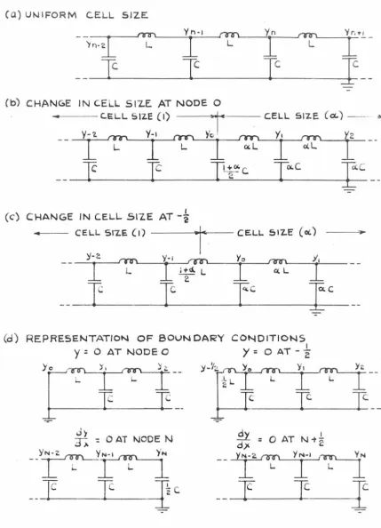
Several circui t s are developed to represent equation

(34), approximating differentiation with respect to x by finite differences in accordance with the principles set forth in Part I of r eference (2 ). These are given in Fig.

4, page 29. In these circui ts, the node voltages are analogous to

cY

.

'l'he circuit embodying uniform cell size (Fig. 4a )

at

may be solved by standard methods.

The difference equations are, from the summation of currents leaving node n,

- Y n+ 1

+

(

2-Z z ) Y n - Y n-1 = 0 ( 41 )

in which

The solution is

Y11 = A cos n8 + B sin n8, ( 42 )

where

z

=

2 sin ~e. ( 43)

With boundary condi tions as given in Fig. 4d, equation (42)

is valid for 1 ~ n ~

N-

1

.

By

writing out the equations of

the circuits of Fig. 4d and defining Y₀ , Y_₁ , YN, and

YN+t by equation (42), this mathematical statement of the boundary equations is obtained:

y ::=: _{0 at 0 Yo= 0}

y

₌

_{0 at} l

Yo+ Y_, 0

-2

-(44 )

dY _

0

dx - at N YN+I

-

YN-1 = 0

dY -= _{O at} 1

YN+I YN 0

N+z-

-

=

2.9

(a) UNIFORM CELL SIZE.

(b)

(c)

(d)

Yn fTlr) Yra1

I

L

r--r

e

_{J __}

-

-CHANGE IN CELL 517..E AT NODE 0

C.ELL srz.E (1) ~, c C.ELL SIZ.E. (a.) - -

-Y-i. _~ Y-1 _f"'l"n

Yo

_rm

y,

_f"l"1I"'\

I

L

I

L

I

o.:L

I

ot. L

I

JC

I

~""c

·

r

e

CHANGE IN CELL 517.E AT-~

CELL srz.E (1)

l

CELL 51Z.E (0(..) Y·

2-rrtn Y·I ~

Yo

r'l)T\ y

I

L

I

l~d.

_L

I

« L

1

r

r

I

C

ic

-REPRESENTATION OF 60UN DARY CONDITIONS

y

=

0 AT NODE 0

y

=

0 AT - ~ I

Yz

I

±

c

-Y·o=

·- L L l:!

r=;

~ i-~-

Y··

~--c

JC __

~

- 0 AT

N-t~

d,x - '"

YN-2. Yr-i-1

L

FIGURE. 4

E.LECTRICAL

NETWORKS FOR THE

EQ d2.y

;:;i.y

[image:33.618.127.556.75.668.2]

Considering the same boundary conditions as in the case of

the continuous beam, the solutions are

(a) Y = 0 at O. Y = 0 at N. Y.,= Am sin mnn:

N m

=

1, 2, 3, .• , N-1 (45)

W01

fil

-

Zm = 2 sin~

2N

(b ) Y = 0 at

o.

dY _{= 0}

dx at N.

y _n = _{A"' sin (2m-l )n}\""C 2N

m

=

1, 2, 3, .• , N

LV ;fLC

=

2 sin (2m-l )11

~ 4N

Except for over-all factors relating time and impedance measurements of the analogous systems,

N 2 LC = a2

Using this relation, the mode frequencies may be compared

with those of the continuous system, and the error due to lumping is determined.

(a )

(b )

w _ 2N sin mTt

"' - a 2N

Sl. n m

n-2Nr

~c.u"" =~-I= -I

Wni.o W"'o m 1t -2N

2N . (2m-l )re

w.,.=a-sin ₄N

· (2m-l )n

sin

sin km

2N

-I

. k,..

-

...

~

=

w ... -I::::. 4N I

W...o W.,.o ( 2m-l )1T - =

sin

2N

k"' -1

2N 4N

k Z km 4

- _{2 4} rn _N2. t _{..,..l...,..9..,..2""""0"""N~4} -•• •

1.6 Unequal Lumping.

Figs. 4b and 4c give circuit analogies of the

(46)

( 47)

(48)

(49)

(50)

(51)

31

Each cell on the right side of the circuit represents a

segment of the physical system which is a. times as long as that represented by a cell on the left side. The method

of section 1.4 can be used to determine the mode frequencies

of circui ts of this t ype.

The circuits of Figs . 4b and 4c are described by two

difference equations. To the left of the change in cell

size

- YI'\-\ + (2-z!l.) Yn - Yn-t\ - 0

Yn = A cos n81 + B sin n81

where

2 sin

i

8, = z

=

u'1/LC.

To the right of the change in cell size

-Yn-t + (2-o.2zZ ) Yn - Yn+1 = 0

Yn = C cos n8z -+ D sin n8₂

where

2 sin ~e

2

=

c.t z

=

ctwl

LC.

Two circuits are considered whi ch have unequal cell

( 52)

( 53)

(54)

(55)

( 56)

(57)

size, and which are analogs of problem (a ) of the preceding

section. Both are constructed from the circuits of Fig. 4,

as follows:

circuit (i)

y = 0

Relative cel l size 1

Change in cel l size

Relative cell size ~

y = 0

circui t (ii)

y

=

0

at O

Relative cell size 1 Change in cell size

Relative cell size ~

y

=

0

l

at -2

at N _i -J.. _z.

Two circuits are also considered which are analogs of

problem (b) of the preceding section, and are constructed

as follows:

circu:i. t (iii )

y

₌

_o

Re la ti ve cell size 1

Change in cell size

Relative cell size Ol

dY - O

dx

-circuit (iv)

y = 0

Relative cell size 1

Change in cell size

Relative cell size ~

dY - O

dx

-at

-N,

at 0

at

_N

_z

at -N _.!..

I Z

at -2 l

at N

_z

- -₂ I

The end conditions are determined from equations (44).

The mathematical descripti on of the change in cell size is

determined by summing current flow from each node not

satisfied by equations ( 52) or ( 55). In circuits ( i ) and

(iii ) ' employing Fig. 4b, this is done for node 0:

-Y_,

+

( l+ « - l+Cl zz _{) Yo}

-

_1.

_{Y1 = 0}

a.

-"2

a.

where

Yo

satisfies both of equations (53) and (56). In

circuits (ii) and (iv), employing Fig. 4c, equations are

written for nodes -1 and O;

-Y_2 + (

r:~

-zz) Y_1 - i+oc Yo= 0

( 58)

( 59)

-

i:

«

y_,

+

(

£:~

-

z

1.

)

Yo - Y1

=

0 (60)

33

(56). By making use of equations (44) and either equation

(58) or equati ons (59) and (60), difference-equati on

solutions, which are implicit solutions for mode

frequen-cies, are obtained as given in Table 8, page 34. In the

case of circuit (i) the details of this procedure are

carried out in Appendix 4. The methods of section 1.4 are

used to determine the first term in the expansion of the

error in mode frequencies, the results of which are given

in Table 9, page 34. Again, in the case of circuit (i),

this procedure is recorded in Appendix 4.

It is not proposed to analyze these results here to

determine optimum circuitry, but merely to list them as an example of the method of solution for mode frequency

11

able 8 Difference Equation Solutions. Unequal Lumping.

Circuit Implicit Solution

( i ) sin ( N,

e

1 + N₂

e

₂ ) -t v sin N₁8₁ cos N z.82 = 0

(i i ) sj_n (N, 8₁ + N₂8₂ )t v cos N,8₁ sin Nz.82 = 0

(iii ) cos 0~, g,

+

Nz8₂ )- v sin

N

,

e

,

sin N₂8z.

=-

0

(iv ) cos ( NI g I + N 2 gz ) +

v

c 0 s N₁

e

₁ cos Nz8₂

=

0

'"'-/f?C 2 · lg 2 . lg

w y l.J'" = z = sin 2 , = Ci. sin 2 ₂

cosle2_ ₁ _ (l 2)(1 '2.

3

+cx.-z

4

_c_o_s--2"'""-e-, - - ot. 8 z

+

128 z + '" )

Table 9 Mode Frequencies of Circuits with Unequal

Lumping

wfLC'

=

_z

₌

_M k ( 1 _+u )

₌

_M k ( ₁

₊

_Ma, _z

₊

_Maz _,.

_{+ ...}

Circuit _al

( i )

~4

{L

_'Y, (1- ai)

+

C(~] k

+

3 ₂ ( 1-<i...'1.) sin

(i i ) _-

k

₂₄

{

_{[ '11}

_{a.2. ]}

(1-

a

2)

+

k - 3 (1-ct't) sin

2

(i i i ) _-

~4

_{{ [ 7, (1- cx.2)}

₊

«:z ]

_k

₊

3 _{( 1-0.1.) sin}

2

(iv )

k

{['1

(1- a.'1) +

_o."-

J

k - 3 ( 1-

cl

)

sin

2

M

=

NI

+

<l. N2.

?;

=

_M

N

,

21; k}

2

7;

k

}

2

1i

k

}

2

'1',

k

}

( i ) and (ii ) : l{rn

=

mit m ::: l,

2

,

3,

...

_'

N,+ N2..

(i i i ) and (iv): _km== 2m-l 'li'

[image:38.617.128.543.91.639.2]

35

II THE EFFECT OF STA'rISTICAL DEVIATION OF 'rHE VALUES OF

THE ELEMENTS

2.1 General

The analyses of Part I are all concerned with the accuracy of solutions. Given a circuit-analogy of a physical or mathematical system, and a statement of what constitutes the answer, they determine what error wil l exist. It is assumed that any time the circuit is constructed in the

computer, each element will be exactly what the circuit diagram prescribes, and the answer, and hence the error, will be the same each time.

Part II is concerned with thB precision of solutions. Considering that the values of the elements are not exactly their nominal values, and that the elements are not iden-tical, i t is apparent that when a circuit is constructed in the computer by selecting computer elements at random,

successive constructions of the same circuit wil l not give identical answers. Even if the elements are set to assigned values with the aid of a meter, their actual values will be subject to a deviation depending on the precision of the meter, and may be treated as if coming from an original population with this precision.

The precision with which an answer is determined depends on the precision of the value of each element in the circuit

and on the extent to which changes in the value of the element

various circuit parameters x 1, Xz, ••• , xNaccording to

the relation

( 1)

and the circuit parameters are selected from populations

with uncorrelated distributions having r.m.s. deviations

<fr

,

0"2 , •••

,

er"'

about means

x:

,

,

x

:l.

, ••• ,

x

.. ,

respect ively,

then f is characterized by a mean

f =-f

(x

1,

x

-z

, .•• ,

:x

"'

)

( 2) and an r.m.s. deviati on

( 3)

i n which the partial derivatives are evaluated at

(x

,

,

. .

.

'

-x.., ) • ( 9) It is assumed that 0-n are small so that the Taylor series expansion of f about f is sufficiently

accurate with only t~e linear terms present.

Determinat ion of the precisi on of answers by equation

(3) does not direct ly require knowledge of the answer, but

i t does require knowledge of the partial derivatives of the

answer with respect to the parameters. Once again eigenvalue

problems are convenient for the determi nation of precision.

Regarding the mode frequencies as answers, the partial

(10)

derivatives can be obtai ned by a method due to Rayleigh.

'l'his method relates i ncrements in mode frequencies to

i ncrements in the potential and kinetic energies associated

with given mode shapes.

Wh_en applied to a conservative electric circuit,

37

Assuming that a particular mode shape, consist ing of node

voltages V, , V2 , • • • , V1, ••• , VN, is known for a given

electrical system, then the maximum instantaneous el

ectro-static energy associated with this mode is

c.

_j V_J ·2

and the maximum instantaneous magnetic energy is W ... =

i

I;

L j I j2 = l

~

V/

2w2 _L.J ~

The terms Vj are the voltages across the elements Cj , Lj ,

( 4)

( 5)

and are determined from t he known voltages Vi . For the pur-poses of this development, any energy associated with

mutual inductances is included in equation (5) by replacing

them in the circuit by equivalent self-inductance. In normal

mode oscillation of an electric circuit, the energy is at

times entirely magnetic, and at other times entirely

electro-static. Thus the normal mode frequency may be determined by equating

W

e

and

W

m

.

z

I:~

2. L;

w

=----L:

cjv/

To determine the partial derivatives of wwith respect

to the circuit parameters Lj , Cj , it is assumed for the

moment that the voltages defining the mode shape, Vi , and hence Vj ,

( 6 )

..;;1

Y1:

~L· _J

The expressions of equations (7) and (8 ) may be used directly in equation (3).

The assumption of unchanged mode shape bears investi-gation. Followi ng Rayleigh's development, (lO) let the norma 1 coordinates of the given system be

¢

1 ,

¢

2, • • • ,

¢

N

•

While considering one mode, the qth, for example, change one of the elements, C.-, for example, by a small amount JlCr . Then i t is shown that the shape of the new normal vibration mode may be expressed as

i n which the 1-·ll 1 _{s are of the same order as}

_J.l

_•

_{However, i t} is shown also that wt as calculat ed by equation (6) has a

( 8)

stati onary value when the mode shape is that of a normal mode. By equation ( 9) the mode sr1ape is changed by terms of order

)!, so that <JJ'L wi 11 experience change of order

JJ.'l.

.

Tbus, in

differentiat ing equation (6) to obtain equations (7 ) and (8 ), taking the l imit ACr-'r' O or ALr - o insures that all change inw is directly due t o the change in the value of the element, and not to the change in mode shape.

39

2.2 The Second Order Eigenvalue Problem

The example considered here is the circuit of

Fig. 4a with

V

=

0

at nodes

0

and

N.

The normal mode sol u-tions are obtained from equau-tions

(45

)

and

(

46),

section 1.5.

Vn = sin mnn

w-W"'

VLc

=

Zm

=

2 sin m1t

2N

m-== 1, 2, 3, •• • , N-1 (10)

( 11)

Considering Ln ... i. to be the inductor connecting nodes n and

n+l, and Vn+!. the vol tage across Ln+.1. , "

~ ~

V

_{h+i -}

V

_{... ,}

_-

V

n

=

s l

.

n m(n+l)« N _ si·n mn

-r

n

Vn+.l

=

2 sin

m

n

cos m ( n+! )1t

z. 2N N

It is necessary to determine the summations employed in

equations (7) and (8 )

S-i nz.

_w-

mntt

₌

₂

CN

~

_VJ . 2. _

=

_

4 sini m'l'C ~ N-l z. m ( n+7:>~ ·1 )« _ 21-\T • ₂

m

rr

L· L 2N L.-J cos N

-

L

sin 211J

J n-= o l\

The details of the surmnations are given in Appendix 5.

Substituting in equations (? ) and (8),

aw -

(I.)

ac .. - -

NC sin1 mr_N 'l\

ow

(lJ 2.

ol.-+!

= -

NL cos m(r_N +-~ )1t ~

It is now assumed that each of the capacitors Cr is

( 12)

(

13

)

(

14

)

(15)

(1

6

)

chosen from a large population having a mean capacitance C

[image:43.617.116.571.76.723.2]

~~=E~L. Equations (15) and (16) may now be substituted in

equation (3).

N

m

=

1, 2, •.• , N-1;

m:

t

t

(

17)

N

m - ₂ (18)

The details of these summations are also given in Appendix

(19)

m

=-

1, 2, ••• , N-1

The result confirms expectation that the deviation of the

mode frequency is proportional to the mode frequency and

the per unit deviation of the elements, and inversely

pro-portional to the square root of the number of cells used.

From equation (50), section 1.5, i t is seen that the

error due to lumping diminishes as

L,

_u

₂

much faster than the

statistical deviation. Tne two effects will be equal when

N is given by

(m41t4

Jj

No

=

432

E.~

(20)

In the California Institute computer, ! will be

approxi-mately .01, if pains are not taken to select special elements.

In this case N0

=

13. l for the first mode. For this number

of cells,

er

t.U Au>.

w

=

w-;-

= .0024 (21)

It is possible that, because of aging, parasitic

effects, or other reasons, the mean of the values of the

41

Ln L + SL. Assuming that

8

c

and SL are smal l compared

wi th C and L, the expressions determined for cr<.V wil l s t i l l

'

apply. However, the mean frequency, w.,.""8w, wil l differ

from the calculated frequency for the circuit,

<.lJ'"

.

2 sin

!'!!!!

Wm+

6w=

2N

i

(

L+ 8 L ) ( C + SC )

8w,..., SL SC

<V;

=

-

2L - 2C _{( 22 )}

2.3 '.fu.e Fourth-01'der Eigenvalue Problem

The problem is that of the simply supported beam,

taken up i n section 1.3. 'I'he circui t is that of Fi gs. la and

lb, wi th supports at nodes 0 and N. The node voltages, Vn ,

given in equation (18 ) of section 1.3, are the same as those in the problem just considered.

v

,,

,

the voltages across the

elements

L

n

,

are determined from Fig. la.

V _{" = si}• _{n , - -}mnn

v" :::=

¢

n+l

-

_¢

_n-i

z

=

Vn = -T I z ·z sin mn1t

=

N

m= l, 2,

.

.

.

'

1

(Vn'i-1 2Vn + Vn-1 T

w

-./LC

sin mn1t

-

,--N-1 (23)

(24)

The last relation is from equation (11) of Appendix 2.

N-1

L:

Cj

v

/

==

C

'E

sin2

m~

n

=

~

N

(25 )

f\'J<I

V.i2 N-1

L:

' 2

L:

sin2 mnn .

_ol

_c

N

v-

-

(1J

c

N

-

2

~

"""'

( 26)

aw_

_-

UJ

sin1 mrtr

ac,. -

NC

w-

( 27 )

OW U,)

sin2 mrrr

OLY

= -

_NL

_N""

( 28 )

2 3 2 2

2, m~ N

O"w

=

_'N8

( €c + E'- ) m::::l,

.

.

.

_'

l'T-1;

2 ( 29 )

a:

'1 - w'l

1 2

E:!) m= N

w -

_W-2

( ~c

+

2 ( 30)

If _{E'c:= ~L= €}

~

~

O-w=c.o

2

N'

m= 1, 2,

.

.

.

'

N-1;

m

:f:

N

2

(31)

O"c.v

=

WE: _~ N

m :=

2

(32)

Except for the possible mode _m

₌

N _{2' the} results are

ident i cal with those for the second order eigenvalue

problem.

From equation (21 ), secti on 1.3, i t is seen that the

error due to lumping is increased, compared with the second

order problem. Here, th~ deviation is less than the error

due to lumping unless N is greater than N0 , where

(

m

4n4)j

No= 108~2 (33)

Aga:i.n taklng m = l, ~ = .OJ.,

N₀

=

20.8 (34)

O"w AW,

Ci) = CR.), ::: .0019 (35)

It is concluded from the examples of these two

sections tti...at the expected deviation of the answer resulting

from the distribution of the element s about their means wil l

be negl igible compared wlth limit ati ons imposed by the

accuracy of the solution. If the number of cells i s less

than N₀ , the error due to lumping overshadows the effect

of deviatj_on of the element values. If the number of

43

within the specifications of the computer operation.

However, the effect of mean error of the values

of the elements, from equation (22 ), may not be negligible,

as it does not decrease as N is increased.

2.4 Distribution of the Elements of the California

Institute Computer.

The elements of the California Inst itute computer

have been measured accurately for purposes of calibration,

and some of the results of these measurements are given in

Table 10, page 44. The capacitors and inductors were

measured with an a.c. impedance bridge at 1000 cycles, and the r esistors with a d.c. bridge. Each capacitor

measure-ment is of a single unit, and is independent of the other

measurements. For use in the computer, each element is

made up of several units of different nominal values, and

the proper capacitance is formed by connecting units whose

capacitance have the correct sum.

The computer inductor elements each consist of three

coils wound on three separate cores. One coil has a large

inductance, one intermediate, and one small. Each coil has

several taps. The coils are connected in series, so that

by various settings of the taps, a wide range of inductance

values is available. The data of Table lO(b) are for

the various tap settings of the larger inductors only. The

uniformity of the r.m.s. deviations is explained by the fact

that each row represents measurements on the same coils and

[image:47.614.123.551.216.716.2]

Table 10. Distribution of the Values of Elements, Cali-fornia Institute of Technology Electric-Analog Computer

(a) Capacitors

In Per Cent of Nominal Value: Nominal

Q,uanti ty Value, Mean R.m.s.

Measured Microfarads Error Deviation

80 .01 2.20% 1.00%

160 .02 .82 .88

80 .05 .19 .60

79 .1 .32 .93

159 .2 -.27 1.26

80 .5 .04 1.08

32 1. 3.10 1.12

32 2. 3.20 .82

(b ) 20 Inductors

In Per Cent of Nominal Value: Nominal

Value, Mean R.m.s.

Henrys Error Deviation

.06 -.30% 1.30%

.12 - • 52 1.24

.18 -.17 1.18

.24 .09 1.18

.30 .25 1.22

• 36 .07 1.16

.42 .86 1.19

.48 .85 1.45

• 54 1.03 1.19

.60 .90 1.19

.66 1.29 1.20

.72 1.24 1. 22

.78 1.25 1.20

.84 1.63 1. 24

.90 1. 95 1.23

[image:48.612.156.529.116.651.2]

45

Table 10. (Continued)

( c ) 7 8 Re s i s t ors

In Per Cent of Nominal Values

Nominal

Value, Mean R.m.s.

Ohms Error Deviat1on

2 6. 7 5;1o 3.62;1o

4 2.82 1.82

6 1. 63 1.23

8 1.01 .90

10 2.43 1.00

20 1.66 .66

30 1.39 • 54

40 1.28 • 52

50 1.23 .50

60 1.14 .42

70 1.10 .41

80 1.08 .39

90 1.06 .37

100 .97 .37

100 .191 • 58

200 .092 .43

300 .020 .36

400 .029 .31

500 .017 .29

600 • 012 .29

700 .024 .28

800 .018 .26

900 .013 .27

1000 -.100 .24

1000 .47 .30

2000 .46 .32

3000 .49 .23

4000 .49 .20

5000 .51 .18

[image:49.614.162.495.118.578.2]