Using the Force: Applications and Implications of Turbulence Forcing Terms in Direct Numerical Simulations

(1)

turbulence forcing terms in direct numerical simulations

Thesis by

Chandru Dhandapani

In Partial Fulfillment of the Requirements for the Degree of

Doctor of Philosophy

CALIFORNIA INSTITUTE OF TECHNOLOGY Pasadena, California

2019

(2)

Chandru Dhandapani ORCID: 0000-0002-7319-557X

(3)

ACKNOWLEDGEMENTS

I would like to thank everyone who has helped me in the past five years, while I was working on and writing my thesis. I would like to thank my advisor Guillaume Blanquart for all the scientific discussions, improving my research quality, and helping me negotiate academic life. I want to thank my thesis committee: Dale Pullin, Dan Meiron, and Tim Colonius, for all the productive discussions about my thesis and the constructive feedback. Thanks to my past members of TheFORCE at Caltech: Simon, Bruno, Brock, Jason, and Nick for all helping me learn the ropes in the group, the code, and the research. Thanks to the present members, Jeff, Rachel, Guillaume, and Joe for the helpful conversations. Thanks to all of you for being my Mind stone.

I would like to thank my Power stone, the Resnick Sustainability Institute and Air Force Office of Scientific Research for financially supporting my research. The GALCIT and MCE staff, the graduate office at Caltech, Laura and Daniel at ISP, Caltech Center for Diversity, and the Caltech Counseling Center also helped me tackle graduate student life in general.

I would like to thank my Space stone, my friends from Indian Institute of Technology, Madras, and Caltech community members from the Indian Subcontinent. You helped me teleport to India figuratively, and I always look forward to our road trips and conversations.

Thanks to my Time stone, the Caltech Glee club, Caltech Dhamaka, TACIT, and IMPLICIT, for enabling my extra-curricular escapades, and helping me feel like an undergraduate student again.

Thanks to my Reality stone, my class of GALCIT engineers that joined in 2014 (and its honorary members), my roommates, GSC, CCA, and GHC. Thanks for keeping me grounded in reality.

And finally, thanks to my Soul stone, to my family: my parents, my siblings, my brother-in-law, and my nephew, Linga, for the joy and support they bring to my life, and the unconditional love they shower me with.

(4)

ABSTRACT

Most energy requirements of modern life can be fulfilled by renewable energy sources, but it is impossible in the near future to provide an alternative energy source to combustion for airplanes. That being said, combustion in aviation can be made more sustainable by using alternative jet fuels, which are made from renewable sources like agricultural wastes, solid wastes, oils, and sugars. These alternative fuels can be used in commercial flights only after a long certification process by the Federal Aviation Agency (FAA) and ASTM International. Unfortunately, in over 50 years of fuel research, only five fuels have been certified. This research project aims to speed up the certification process with quicker testing of alternative fuels. Engine testing and even laboratory testing require large amounts of time and fuel. Simulations can make the process much more efficient, but accurately simulating highly turbulent flames in such complex geometries would need large amounts of computational resources. The goal of this thesis is to create an efficient computational framework, that can replicate different engine-like turbulent flow conditions in simple geometries with numerical tractability.

The central idea is to decompose the flow field into ensemble mean and fluctuating quantities. The simulations then resolve only the fluctuations using simple com-putational domains, while emulating the effect of the mean flow using "forcing" terms. These forcing terms are calculated first for incompressible turbulence, and this method is later extended to turbulent reacting flows. In incompressible turbu-lence, Direct Numerical Simulations (DNS) performed on simple triply periodic cubic domains reasonably capture the statistically stationary shear turbulence, that is observed in free shear flows. The simulations are also performed in cuboidal domains, that are longer in one direction and with an inflow/outflow along it. Both changes are observed to not have a significant impact on the turbulence statistics. Fi-nally, shear convection is applied to the turbulence simulations with inflow/outflow, which has a significant impact on the turbulence. These simulations accurately capture the turbulence anisotropy in free-shear flows.

(5)

(6)

PUBLISHED CONTENT AND CONTRIBUTIONS

[1] C. Dhandapani, K. J. Rah, and G. Blanquart. “Effective forcing for direct numerical simulations of the shear layer of turbulent free shear flows”. In: Physical review fluids (accepted for publication)(2019).

(7)

LIST OF ILLUSTRATIONS

Number Page

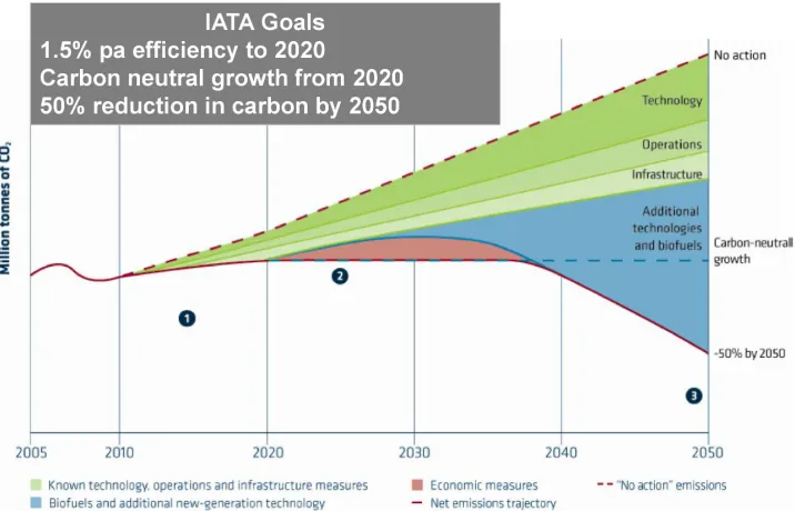
1.1 CO2 emissions reduction roadmap of International Air Transport Association (IATA). Major contribution to CO2 reduction is from alternative fuel technology, and more effective than improvement in Operations, Infrastructure and Technology. Source : International Air Transport Association (IATA) . . . 2 1.2 Combustion chamber of a turbojet engine . . . 3 1.3 a) Experimental setup of a turbulent reacting jet at the CFRL in USC

b) LES results of a turbulent reacting jet – Temperature Contours c) DNS results of a turbulent flame – Temperature contours. . . 8 2.1 Different turbulent free shear flows considered for the current study

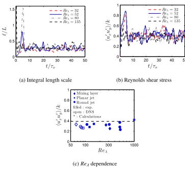
with the computational domain chosen (red cube): a) nearly homo-geneous shear turbulence (NHST) b) mixing layer (ML) c) planar jet (PJ) d) round jet (RJ). . . 14 2.2 a) Integral length scale normalized by the domain width, b) Reynolds

shear stress hu0_xu0_yi normalized by turbulent kinetic energy, for the four DNS, and c) comparison of Reynolds number dependence of Reynolds shear stress hu0xu0yi with other studies. Dashed lines cor-responds to the averaged value obtained from all simulations in the current study. . . 24 2.3 a) Turbulent kinetic energy normalized by its expected value (Eq. 2.39).

b) Energy dissipation rate normalized by its expected value (Eq. 2.40). c) Taylor microscale Reynolds number,Reλ, for DNS 3. Dashed line corresponds toReo_λ =80. . . 28 2.4 a) Rms velocity components along x, y, andz, normalized by urms,

(10)

2.5 Comparison of one-dimensional energy spectra along xandz direc-tions. R & M refers to the energy spectra published by Rogers and Moser [70]. . . 34 2.6 a) Energy spectra normalized by ε and ν. b) Shear stress spectra

normalized by ε and ν. The dashed line corresponds to turbulence scaling from literature,κ−5/3in a) andκ−7/3in b). . . 34 2.7 Normalized turbulent kinetic energy budget. The lines correspond

to experimental results from Panchapakesan and Lumley [59]. Symbols correspond to different simulations: DNS3 circles, DNS 3a -triangles, DNS 3b - squares. . . 36 2.8 Ratio of production to dissipation of kinetic energy. The blue line

corresponds to simulations in the current study and the three lines correspond to three simulations by Kasbaoui et al., with different initial conditions. . . 37 2.9 Joint pdf of the normalized velocity fluctuations in the x and y

direc-tions from simulation with a) just the off-diagonal term, and b) linear and non-linear terms. . . 38 2.10 Marginal pdf of the normalized velocity fluctuations in the a) xand

b) ydirections from simulation with just the off-diagonal term, and linear and non-linear terms. . . 39 2.11 Evolution of turbulent kinetic energy normalized by the expected

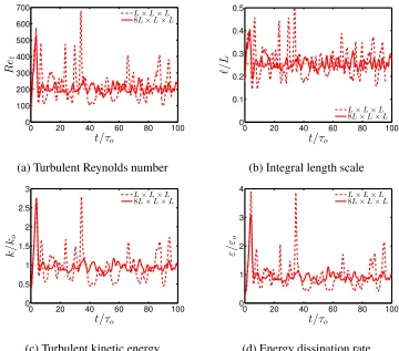
value (Eq. 2.39) for different treatment of the shear convection term. . 41 3.1 Isotropic turbulence simulation results. Time evolution of the

tur-bulent Reynolds number (a), integral length scale normalized by the domain width L (b), turbulent kinetic energy normalized by the ex-pected values, ko,i, (c) energy dissipation rate normalized by the

expected values, εo,i (d) for cubic (dashed lines) and cuboidal

(11)

3.2 Shear turbulence simulation results. Time evolution of the turbulent Reynolds number (a), integral length scale normalized by the domain width L (b), turbulent kinetic energy normalized by the expected values, ko,i, (c) energy dissipation rate normalized by the expected

values, εo,i (d) for cubic (dashed lines) and cuboidal domains (solid

lines). Dotted lines and dash-dotted lines in a) and b) represent the average values from the cubic and cuboidal simulations respectively. . 49 3.3 Time evolution of Reynolds shear stress normalized by the turbulent

kinetic energy. . . 50 3.4 Advection velocity profile normalized by the shear forcing constant

and domain width. . . 52 3.5 a) Turbulent Reynolds number profile, b) Integral length scale

nor-malized by the domain width, c) Turbulent kinetic energy profile normalized by the expected value ko, d) Energy dissipation rate nor-malized by the expected value εo, for isotropic (blue) and shear forcing (red) cases. Dashed lines in b) correspond to average values. . 53 3.6 Velocity fluctuation magnitudes for the isotropic forcing (a) and shear

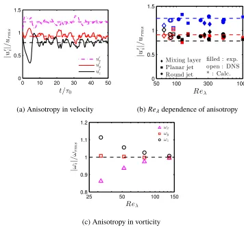
forcing (b), normalized by the root mean square velocity,urms. Vor-ticity fluctuation magnitudes normalized by the root mean square ve-locity,ωrms, for the isotropic forcing c) and shear forcing d). Dashed lines in (b) correspond to average values. . . 54 3.7 Reynolds shear stress profile normalized by the turbulent kinetic energy. 55 3.8 a) Turbulent Reynolds number profile, b) Integral length scale

nor-malized by the domain width, c) Turbulent kinetic energy profile normalized by the expected value,ko, d) Energy dissipation rate nor-malized by the expected value, εo, for isotropic (blue), shear (red), and advection (black) cases. . . 57 3.9 Velocity fluctuation magnitudes for the shear simulation (a) and

ad-vection simulation (b), normalized by the root mean square velocity,

(12)

3.11 a) Anisotropy in velocity from other studies of free shear flows as a function of Reynolds number for u0x (red), u0y (blue), and u0z (black)

b) Reynolds shear stress values as a function of Reynolds number. Dashed lines correspond to the portion with the shear convection included from the advection case. . . 59 3.12 Normalized turbulent kinetic energy budget. The lines correspond

to experimental results from Panchapakesan and Lumley [59]. Sym-bols correspond to different simulations: Incompressible with shear convection diamonds, Chapter 2 results: DNS 3 circles, DNS 3a -triangles, DNS 3b - squares. . . 60 4.1 Reacting jet schematic, with unburnt mixture represented in blue,

flame location in yellow, and burnt mixture in red. The black cuboid marks the simulation domain, with the Cartesian directions of the domain indicated. . . 62 4.2 Velocity decomposition of the instantaneous velocity field, u, into

the imposed scales,ui, and the resolved scales,ur. . . 65 5.1 Advection velocity profile normalized by the shear forcing constant

and domain width. . . 74 5.2 Schematic of the computational domain for the turbulent flame

sim-ulations, adapted from Savardet al.[19] . . . 76 5.3 Instantaneous temperature contours in the x-y plane for isotropic

forcing (top) and shear forcing (bottom). The black curves locate the edges of the reaction zone, corresponding to Tpeak −30K and

Tpeak+30K, whereTpeakis the maximum fuel consumption temperature. 79 5.4 a) Turbulent kinetic energy profile normalized by the expected value

ko, b) Energy dissipation rate normalized by the expected value εo, and c) Integral length scale normalized by the domain width for isotropic (blue) and shear forcing (red) cases. . . 80 5.5 a) Turbulent Reynolds number profile and b) Karlovitz number profile

for isotropic (blue) and shear forcing (red) cases. . . 81 5.6 Time evolution of the turbulent flame speed normalized by the laminar

(13)

5.7 a) Conditional mean of fuel and hydrogen mass fractions versus temperature, b) Conditional mean of fuel consumption rate versus temperature, c) Probability density function of fuel consumption rate at maximum fuel consumption temperature,Tpeak. . . 82 5.8 Velocity fluctuation magnitudes for the isotropic forcing (a) and shear

forcing (b), normalized by the root mean square velocity,urms. Vor-ticity fluctuation magnitudes normalized by the root mean square vorticity, ωrms, for the isotropic forcing (c) and shear forcing (d). The gray dashed lines correspond to the edges of the flame brush, xs

and xe, wheredρ/dxreaches its minimum value at 0.5(xs+ xe), and

xe− xs = (ρb− ρu)/(dρ/dx)_min . . . 83 5.9 Reynolds shear stress normalized by the turbulent kinetic energy for

isotropic (blue) and shear (red) cases. . . 84 5.10 Instantaneous temperature contours in the x-y plane for shear

sim-ulation (top) and advection simsim-ulation (bottom). The black curves locate the edges of the reaction zone, corresponding toTpeak−30K and Tpeak + 30K, where Tpeak is the maximum fuel consumption temperature. . . 86 5.11 a) Turbulent kinetic energy profile normalized by the expected value

ko, b) Energy dissipation rate normalized by the expected value εo, and c) Karlovitz number profile for isotropic (blue), shear (red), and advection (black) cases. . . 86 5.12 Time evolution of the turbulent flame speed normalized by the laminar

flame speed (a) and turbulent flame surface area normalized by the cross-section area (b) for shear (red) and advection (black) simulations. 87 5.13 a) Conditional mean of fuel and hydrogen mass fractions versus

temperature, b) Conditional mean of fuel consumption rate versus temperature, c) Probability density function of fuel consumption rate at maximum fuel consumption temperature,Tpeak. . . 88 5.14 Velocity fluctuation magnitudes for the isotropic forcing (a) and shear

(14)

5.15 Instantaneous temperature contours in thex-yplane for the isotropic case (top) and pressure case (bottom). The black curves locate the edges of the reaction zone, corresponding toTpeak−30KandTpeak+ 30K, whereTpeakis the maximum fuel consumption temperature. . . 90 5.16 a) Turbulent kinetic energy profile normalized by the expected value,

ko, b) Energy dissipation rate normalized by the expected value,

εo, for isotropic (blue), shear (red), advection (black), and pressure (magenta) cases. The gray dashed lines correspond to the edges of the turbulent flame brush. . . 91 5.17 a) Turbulent kinetic energy budget profile - Production (blue),

pres-sure term (blue), advection (green), dissipation (magenta), and sum (black). b) Karlovitz number profile for isotropic (blue), shear (red), advection (black), and pressure (magenta) cases. . . 91 5.18 Time evolution of the turbulent flame speed normalized by the laminar

flame speed (a), flame surface area normalized by the cross section area (b), and burning efficiency factor (c). Dotted lines correspond to the average values. . . 92 5.19 a) Conditional mean of fuel and hydrogen mass fractions versus

temperature, b) Conditional mean of fuel consumption rate versus temperature, c) Probability density function of fuel consumption rate at maximum fuel consumption temperature,Tpeak. . . 93 5.20 Velocity fluctuation magnitudes for the isotropic simulation (a) and

pressure simulation (b), normalized by the root mean square velocity,

urms. Vorticity fluctuation magnitudes normalized by the root mean square vorticity,ωrms, for the isotropic case (c) and pressure case (d). The gray dashed lines correspond to the two edges of the turbulent flame brush. . . 94 5.21 Reynolds shear stress normalized by the turbulent kinetic energy for

isotropic (blue), shear (red), advection (black), and pressure (ma-genta) cases. . . 95 6.1 Plan of attack for bio-fuel testing. . . 100 6.2 a) Velocity fluctuation magnitude profiles and b) Turbulent kinetic

energy budget as a function of the radial distance,r. . . 101 6.3 a) Progress variable contours and b) Enstrophy (ω2) contours. . . 102 A.1 Two-dimensional representation of the discretization of the

(15)

LIST OF TABLES

Number Page

2.1 Simulation parameters of the different cases of shear turbulence sim-ulations . . . 27 2.2 Results from shear turbulence simulations in triply periodic cubic

simulations . . . 29 2.3 Anisotropy results from various experiments and simulations of

dif-ferent free shear turbulent flows. Average values of u0_i/urms and hu0xu0yi/k in the middle of shear layers of ML (mixing layers), PJ (planar jets), and RJ (round jets). S corresponds to simulations, E corresponds to experiments, C corresponds to calculations. . . 30 2.4 Turbulence quantities before and after shear remapping. . . 40 3.1 Simulation parameters of the triply periodic domain simulations. . . . 44 3.2 Scaling parameters of the incompressible turbulence simulations. . . 46 3.3 Simulation parameters of the three different cases of incompressible

turbulence with inflow/outflow . . . 50 5.1 Simulation parameters of the different cases of turbulent flame

(16)

C h a p t e r 1

INTRODUCTION

1.1 Background

Humanity as a whole has been moving away from fossil-fuels and towards renewable energy sources such as solar, wind, and water energy. These renewable sources of energy can be used for power generation, land transport, heating etc. Electric cars and trains are already in commercial use and electricity generation has been relying less on fossil fuels. In fact, most energy requirements of modern life can be fulfilled by clean energy sources, but not all of them. The high energy density required for air transport can only be met by combustion. In other words, we are “stuck with combustion” for airplanes. The question then becomes can we make combustion in airplanes more sustainable?

Commercial airplanes use petroleum-based jet fuel for combustion, which leads to high CO2 emissions. Aviation industry accounts for 12% of CO2 emissions from transportation. As Fig. 1.1 shows, if left unchecked, CO2 emissions from aviation will be doubled by 2050. Reductions in CO2emissions could be made by changes in technology, operation and infrastructure, but that still will not be enough to decrease emissions. The only way to reduce CO2 emissions to the point of carbon-neutral growth, or even further reduction by 50% of today’s quantity is through a change in aviation fuel. Various organizations have recommended alternative jet fuels, that are not only sourced from renewable sources, but also produce lower CO2 emissions. These alternative fuels could reduce the carbon-footprint of aviation by up to 80% over the full lifecycle (production, refining, transportation and combustion).

(17)

[image:17.612.133.491.80.310.2]

Figure 1.1: CO2 emissions reduction roadmap of International Air Transport As-sociation (IATA). Major contribution to CO2 reduction is from alternative fuel technology, and more effective than improvement in Operations, Infrastructure and Technology. Source : International Air Transport Association (IATA)

far, five alternative jet fuels have been approved by the FAA:

1. Alcohol to Jet Synthetic Paraffinic Kerosene (ATJ-SPK) synthesized from alcohols obtained from fermentation of biomass,

2. Synthesized Iso-Paraffins (SIP) produced from sugars,

3. Hydro-processed Esters and Fatty Acids Synthetic Paraffinic Kerosene (HEFA-SPK) made from hydrotreating virgin or waste oils,

4. Fischer-Tropsch Synthetic Paraffinic Kerosene (FT-SPK), and

5. Fischer-Tropsch Synthetic Kerosene with Aromatics (FT-SKA). FT-SPK and FT-SKA are obtained by pyrolysis/gasification and processing of biological wastes.

(18)

The procedure involves testing fuels in engine-scale tests, completely oblivious to the dependence or independence of turbulent combustion on fuel-specific properties. The certification process fails to utilize existing knowledge of turbulent combustion, and the inherent connections between turbulent and laminar flames.

Combustion in engines depends on engine-specific physics and engine-independent characteristics that are common to all turbulent flames. In turn, turbulent flame properties can be further classified into fuel-specific chemistry and fuel-independent properties. Of these fuel-specific properties, engine combustion would only depend on a small subset of laminar flame parameters of the fuel [48]. The goal is to identify these laminar flame properties that significantly affect turbulent flame behavior, and test new fuels for only this small set of parameters to make sure that the alternative fuel behaves like ATF in engines.

Figure 1.2: Combustion chamber of a turbojet engine

1.2 From engine experiments to direct numerical simulations

Full engine tests: Commercial aircraft engines are either turbojet, turboprop, or turbofan engines, which all contain a compressor stage, a combustion chamber, and a turbine stage in that sequence. The fuel is premixed with compressed air and introduced into the chamber in jets and ignited (see Fig. 1.2). Engine combustion occurs in strongly turbulent conditions, which enhance both mixing and combustion and improve the energy efficiency. These highly turbulent flows can be easily replicated in engine tests, but the tests would consume large amounts of fuel (0.5 to 3 kg/s). Acquiring or processing such large amounts of fuel might not be feasible for alternative jet fuels at the testing/certification stage.

(19)

the high shear turbulent combustion found in jet engines (see Fig. 1.3a). These laboratory setups include reacting jets [55, 54, 5, 61], nozzle type burners [46], reacting shear layers [56], turbulent V-flames, swirl burners [6], backwards facing step, jets in cross flow [43], and bluff-body stabilized flames [4]. These experiments use smaller amounts of fuel (0.1 to 1.5 g/s) and are ideal for testing commonly available fuels. Researchers have studied such turbulent flames, with different fuels, over a wide range of equivalence ratios and turbulence intensities. But the fuel requirement may still be too high for potential alternative jet fuels which are not in the phase of mass-production.

Laminar combustion experiments: Aviation turbine fuel and sustainable alter-natives to it are all long chain carbon fuels, the combustion of which involves tens of different species and hundreds of elementary chemical reactions. The exact chemical composition and the laminar combustion behavior of the fuel can be easily measured with very small amounts of fuel in simple laboratory settings [33, 39, 42, 83, 91].

(20)

LES and RANS: Computational costs can also be reduced by performing large eddy simulations (LES) which use coarse grids to capture large scale flow effects [82, 8], and use sub-grid scale models for the unresolved small scales [63, 26, 62]. While these simulations can capture the large scale behavior of the reacting flow with reasonable accuracy, fuel-specific chemical reactions and their interactions with turbulence occur at small scales, that are not fully captured by these simulations [11]. Reynolds Averaged Navier Stokes (RANS) methods work in a similar fashion, where the ensemble mean velocity field is solved for, while the Reynolds stress and scalar flux terms are estimated using different RANS models [12, 87]. Despite recent developments [47, 85], there is still a need for extensive research and higher fidelity in closure models for reacting flows for both LES and RANS.

Small region DNS: Some computational studies cut down on computational do-mains by performing fully resolved DNS of turbulent flames in simple geometries. However, most of these simulations are not statistically stationary, which is not ideal for steady state observations. For instance, Rutland and Trouve performed simu-lations of outward propagating flames in triply periodic cubic domains, containing decaying isotropic turbulence [73]. Gruber et al. observed turbulent flame-wall interactions in decaying channel flow turbulence [34]. Hamlingtonet al. performed turbulent flame simulations using isotropic turbulence, with the turbulence sustained by introducing random perturbations in the largest scale of the flow. Multiple stud-ies from TheFORCE lab at Caltech have simulated statistically stationary turbulent flames, using linear isotropic forcing to sustain turbulence [75, 76, 49, 9, 48, 79, 78]. The velocity fields in these simulations either contain decaying turbulence, or maintain constant turbulence using artificial numerical methods. This status quo comes from the fact that the large scale flow effects observed in larger domains are missing in such simulations, and one of the effects of the large scale flow is main-taining constant turbulence statistics over time. Ideally, one would like statistically stationary simulations which can accurately reflect the turbulence and can capture the large scale flow effects observed in different experimental setups for turbulent reacting flows.

(21)

captured, the targeted method should do the opposite. The small-scales/fluctuations are fully resolved in the simulations, while "forcing" terms are introduced to emulate the impact of the large-scale/mean flow.

These frameworks need to be tested for both incompressible turbulence and turbulent flame simulations.

1.3 Incompressible turbulence

Turbulent free shear flows are found in a multitude of industrial applications and in nature, and their analysis gives a lot of insight into turbulence and its structure. However, owing to the range of scales and the stochastic and unsteady nature of turbulence, even simulating such incompressible flows has proven to be quite challenging. Various configurations have been used to simulate turbulent flows using DNS, that are resolved down to the smallest turbulent length scales. The different DNS methodologies can be broadly classified into three major configurations.

The most obvious configuration is to use the entire domain to solve the spatially evolving flow [86, 10, 88]. In this configuration, the turbulence statistics reach a sta-tionary state after a transient period, and hence the results are ultimately independent from the initial conditions. Unfortunately, the overall flow field depends strongly on the boundary conditions. These simulations typically include a near-field region where the turbulence is not fully developed, and so this configuration is not compu-tationally efficient. Since the entire flow field needs to be solved, these simulations are usually performed at lower Reynolds numbers to reduce the computational costs.

Another configuration is to perform temporally evolving turbulent flow simulations. A perfect example is the mixing layer simulation by Rogers and Moser [70], which introduces homogeneity in the streamwise direction. The extra periodic direction increases the computational efficiency, but does so at the expense of physics. It also aids in calculating the energy spectra, which can be used to observe the different scales of turbulence. Unfortunately, the statistics never reach a stationary state, and hence the results still depend heavily on the initial conditions.

(22)

viscous dissipation [38]. Hence, to keep the turbulent kinetic energy stationary over time, the missing mean shear needs to be emulated through a method of forcing the turbulence. Turbulence in the past has been forced by different techniques, including spectral forcing [28, 32, 17, 23] and linear forcing [53, 72, 20]. While these techniques are required to generate turbulence in the domain, these numerical forcing techniques have been mostly arbitrary, and do not capture the physics of the large scale flows accurately.

Recently, Rah et al. [67] combined the numerical tractability of the third config-uration with the physical accuracy of the first configconfig-uration. They used a triply periodic computational domain, with the forcing calculated from the flow physics at a small region at the centerline of a turbulent round jet, and forced turbulence in a mathematically consistent way. The current study extends this work by consider-ing a small region in the self-similar shear layer of multiple statistically stationary free-shear flows and using a triply periodic computational domain to simulate this shear-dominated flow.

Several homogeneous shear turbulence (HST) simulations have been performed in the literature using similar techniques [69, 31, 50, 14, 41, 45, 80]. While a shear production term was included in each study, considering an idealized homogeneous shear flow, the forcing terms were not derived for practical turbulent flows, and ultimately lacked the mathematical background to be compared to realistic turbu-lent flows. Most of these simulations used shear periodic boundary conditions, but simulate idealized homogeneous shear flow, and the turbulence statistics grow ex-ponentially in time [31, 50, 14, 41, 45]. Other simulations include a wall boundary in the cross-stream direction, and are not homogeneous [80].

It is also important to remember that these simulations aim to capture the velocity fluctuations observed in statistically stationary free-shear flows. As a consequence, these simulationsneed to have stationary statistics, and be stable enough for simu-lations over long periods of time.

1.4 From incompressible to flame simulations

(23)

from the domain at a steady rate. This can accomplished by foregoing periodic boundary conditions in the flame normal direction, and introducing an inflow on the reactants side and a convective outflow on the side of the products. These boundary conditions create non-homogeneity in the flame-normal direction, and can also have an impact on the flow near the inflow/outflow.

In addition, when introducing an inflow/outflow, the domain width needs to be higher in the direction of the inflow/outflow, so that the boundary conditions do not affect the turbulence statistics in the domain, away from the inlet/outlet. Furthermore, it is desirable for the turbulence to be fully developed before reaching the flame front. Hence, the computational domains for these simulations need to be much longer along one direction. Changing the aspect ratio of the computational domain may affect the simulation results, and these effects need to be studied in detail. As an added benefit, the non-homogeneous direction in the simulation with inflow/outflow allows for studying the effects of shear convection, which is present in free-shear flows of both incompressible and reacting turbulence.

[image:23.612.120.496.433.639.2]

All these impacts need to studied using incompressible flows, before chemistry can be included in the simulations. Once these large scale effects are accurately under-stood and quantified in incompressible simulations, turbulent flame simulations can be performed using a similar methodology.

(24)

1.5 Turbulent flames

One should be careful in extending these turbulence simulation techniques to react-ing flames, as turbulent flames involve the complex interaction between two non-linear processes: turbulence and combustion. The mean flow is affected both by the flow geometry and the chemical reactions. Despite these difficulties, turbulent flame simulations focusing on velocity fluctuations can be found in the literature. Several studies have reduced the computational cost by considering a small region of the turbulent flame and performing DNS with the same turbulence parameters [3, 76, 49, 36]. These simulations consider canonical three-dimensional domains that are often periodic in two directions with the flame progressing along the non-periodic direction, as seen in Fig. 1.3c. This approach offers high-fidelity simulations at low computational costs, and the periodic boundaries help in eliminating boundary condition effects on the simulations.

The disadvantage to these simulations is that the large scale flow effects are not captured. One of the missing effects is the mean shear that generates turbulence, and hence the turbulent kinetic energy decays over time due to viscous dissipa-tion [18, 19]. This is tackled by implementing numerical turbulence forcing in the simulation [36, 2], to keep the turbulent kinetic energy statistically stationary over time.

Several forcing methodologies have been used [36, 2, 64, 75, 49, 76, 72] in past studies. Some turbulence forcing techniques are applied only to low wavenumbers and some are implemented over all scales. Some studies use forcing techniques that are in correlation with the velocity and some forcing methods are not correlated with the velocity field. The forcing term can be applied in spectral space or in physical space, linear with velocity. However, one common factor across all all these numerical forcing schemes is that they have been mostly arbitrary. Most forcing methods generate isotropic turbulence and they do not reflect the flow physics observed in turbulent reacting flows.

The current study aims at mathematically deriving the exact turbulence forcing technique that is physically consistent and compatible with the large scale flow physics and reflects the turbulence observed in turbulent flames. The forcing term comes directly from the turbulence production, that is calculated from the gradients of the large scale velocity. This turbulence production technique will be compared against the isotropic forcing scheme suggested by Lundgren [53].

(25)

scale flow effects are missing. The turbulence production term is often the source of inspiration for the forcing terms, while the other impacts of the large scale flow can be emulated in the DNS using such similar forcing terms calculated from the large scale flow. The large scale effects like the impact of a mean pressure gradient and shear convection on the turbulent flame behavior are also studied.

Researchers in the past have studied turbulent behavior and their dependence on different factors: fuel type [48], equivalence ratio [48], differential diffusion [49], thermal diffusion [78], turbulence intensity [76, 51], combustion models [79], etc, and most of these studies have been performed with isotropic simulations, with no other large scale effects reflected in the simulations. The impact of the anisotropy of the turbulence and the different flow conditions on the turbulent flame behavior needs to be observed, so one can know if it is reasonable to compare experiments of turbulent flames with different configurations against each other, and against idealized isotropic turbulence simulations.

1.6 Outline

The goal of this thesis is to study the effects of different turbulent flow conditions on the velocity and scalar statistics of turbulent flames. This is achieved by following the research plan given below:

1. Develop a mathematical framework to simulate portions of the incompressible turbulent flow field by using a RANS-inspired velocity decomposition and simulating only the fluctuating quantities.

2. Recreate the statistically stationary shear turbulence observed in free shear flows in homogeneous domains.

3. Extend the simulations to other computational domains to study the impact of aspect ratio, non-homogeneity, and boundary conditions on isotropic and shear turbulence

4. Analyze the effects of shear convection on shear turbulence and its anisotropy.

5. Extend the mathematical framework to variable density flows with chemistry effects and scalar transport.

(26)

7. Analyze the impact of favorable pressure gradients and shear convection on the turbulent flames.

(27)

C h a p t e r 2

EFFECTIVE FORCING FOR DIRECT NUMERICAL

SIMULATIONS OF THE SHEAR LAYER OF TURBULENT

FREE SHEAR FLOWS

[1] C. Dhandapani, K. J. Rah, and G. Blanquart. “Effective forcing for direct numerical simulations of the shear layer of turbulent free shear flows”. In: Physical review fluids (accepted for publication)(2019).

2.1 Introduction

A numerically efficient configuration to simulate turbulent flows is to use triply periodic domains, with numerical forcing techniques to sustain turbulence. Previous homogeneous shear turbulence simulations considered only idealized homogeneous shear flows, and not the statistically stationary shear turbulence observed in practical free shear flows. In contrast, the current study mathematically derives the complete forcing technique from the large scales of the turbulent free shear flows. Different statistically stationary free shear flows are considered in this study, namely a nearly homogeneous shear turbulent flow, turbulent mixing layer, a turbulent planar jet, and a turbulent round jet. The simulations are performed on triply periodic, statistically homogeneous cubic domains in the vicinity of the shear layer in the self-similar region. An a priori analysis is performed to calculate the effects of the different forcing terms and to predict the expected turbulence quantities. The tailored forcing technique is then used to perform direct numerical simulations at different Reynolds numbers. Numerical results for the different cases are discussed, and compared with results from experiments and other simulations of free shear turbulent flows.

(28)

2.2 Mathematical derivation

We start by reviewing Lundgren’s mathematical approach, which uses a Reynolds decomposition to identify the effects of the large turbulent scales on the small scales. Then, four canonical flows are considered (see Fig. 2.1), and the forcing matrix is calculated for each of them. A forcing technique, common to the self-similar shear layer of these four flows, is discussed after.

2.2.1 Methodology : Review of Lundgren’s approach

First, we consider the Navier-Stokes (NS) equations for the velocity field u for a fluid flow with constant density ρ, where p is the pressure and ν is the kinematic viscosity,

∂u

∂t +u· ∇u =−

1

ρ∇p+ν∇2u. (2.1)

For any turbulent flow phenomenon, the instantaneous velocity field can be de-composed into mean and fluctuating velocity fields (i.e., Reynolds decomposition),

u= u+u0, where · represents the ensemble average. Transport equations for the fluctuations are obtained by calculating the difference between the NS equations for the full velocity field and the transport equations for the mean velocity field, namely

N S(u+u0) −N S(u+u0₎. _(2.2)

This leads to

∂u0

∂t +(u+u

0_{) · ∇}

u0=−1

ρ∇p

0₊_ν_∇2_u0₊_{∇ ·}

u0_u0₋_u0_{· ∇}

u. (2.3)

The extra terms in the transport equations for the fluctuating velocity, when compared with Eq. (2.1), are the mean-flow advection term (u· ∇u0), the divergence of the Reynolds stress term (∇ ·u0u0), and the production term (−u0· ∇u). Lundgren focused on the production term as the only contributor to turbulent kinetic energy production [53], but this is not the case as will be seen later in section C. The major contribution to the turbulent kinetic energy comes from the production term, which is rewritten as a forcing termA·u0,

∂u0 ∂t +u

0_{· ∇}

u0=−1

ρ∇p

0₊_ν_∇2_u0₊

A·u0, (2.4)

where A is the forcing matrix, given by A = −∇u. The source term is linear in

(29)

(a) NHST (b) ML

[image:29.612.152.462.66.337.2]

(c) PJ (d) RJ

Figure 2.1: Different turbulent free shear flows considered for the current study with the computational domain chosen (red cube): a) nearly homogeneous shear turbulence (NHST) b) mixing layer (ML) c) planar jet (PJ) d) round jet (RJ).

Lundgren [53] further assumed that the forcing matrix,Ais a diagonal matrix that generates isotropic turbulence,

ALundgren =

           

A 0 0

0 A 0

0 0 A

           

. (2.5)

This isotropic forcing term was implemented asAu0, where Ais an arbitrary forcing constant, calculated based on the required turbulent Reynolds number [20]. In practice, the forcing matrix depends on the gradients of the mean velocity.

2.2.2 Mean velocity gradients

(30)

homogeneous cubic domains in the vicinity of the shear layer in their respective self-similar region as shown in Fig. 2.1.

2.2.2.1 Nearly Homogeneous Shear Turbulence

For a homogeneous shear turbulence flow, the mean flow is in the streamwise direction(x). The free-stream velocity is constant along x and varies linearly in y, away from the walls located aty =−h/2 andy = h/2. The mean streamwise velocity at the center of the wind tunnel, y = 0 isUC. Far downstream, the quantities are self-similar and are homogeneous in theydirection away from the walls. However, the integral length scale ` increases linearly with x [21], and consequently, the Reynolds stresses and the velocity fluctuation magnitudes increase with x, hence the name “nearly" homogeneous shear turbulence. Equation (2.3) for the HST flow in the center of the wind tunnel becomes,

∂u0 ∂t +u

0_{· ∇}

u0=−1

ρ∇p

0₊_ν_∇2_u0₋ ∂ux

∂y u

0 yex

−ux∂u

0

∂x + ∂u0

xu0x ∂x ex+

∂u0

xu0y

∂x ey. (2.6)

Most simulations of homogeneous shear turbulence use periodic boundary condi-tions in the x direction without rescaling the velocity, and choose to neglect the divergence of the Reynolds stress terms. The forcing matrix for NHST at y= 0 is

AN HST = −

           

0 ∂ux

∂y 0

0 0 0

           

= BN HST            

0 1 0

0 0 0

            . (2.7)

The only element of the forcing matrix is due to the shear strain rate ∂ux

∂y , and the matrix is normalized by that quantity.

2.2.2.2 Mixing Layer

For a spatial mixing layer, the mean flow is primarily in the streamwise direction (x). The freestream velocity is constant along x, and is 0 for y → +∞ and US

(31)

thicknessδ increases linearly withx, and y1/2is linear in x[22]. There is no mean flow in the spanwise direction(uz =0)and the flow is statistically homogeneous in the spanwise direction(∂ux

∂z =0 and

∂uy

∂z = 0).

Equation (2.3) at the center of the mixing layer becomes,

∂u0 ∂t +u

0_{· ∇}

u0=−1

ρ∇p

0₊_ν_∇2_u0₋ ∂ux

∂x u

0

xex

− ∂ux

∂y u

0 yex−

∂uy

∂x u

0

xey− ∂uy

∂y u

0

yey −ux ∂u0

∂x −uy ∂u0

∂y

+ ∂u0xu0x ∂x ex+

∂u0

xu0y

∂x ey. (2.8)

The forcing matrix for the spatial mixing layer at y= y1/2is

AM L =−

            

∂ux

∂x

∂ux

∂y 0

∂uy

∂x

∂uy

∂y 0

0 0 0

            

= BM L            

−0.035 1 0

−0.001 0.035 0

0 0 0

            , (2.9)

calculated from the mean velocity profile given by Lumley [52]. The largest element of the forcing matrix is due to the shear strain rate ∂ux

∂y , and the matrix is normalized by BM L =−∂ux

∂y (y1/2)= 1.022

US

δ .

2.2.2.3 Planar Jet

In a planar jet, the mean flow is primarily in the streamwise direction(x), and the centerline mean velocity at the jet axis,Uo(x), decays alongxas 1/√x[13, 35, 65, 86]. The mean velocities are self-similar far from the jet exit, and when normalized by the centerline velocity, are only functions of the similarity variable,η ≡ y/y₁/2(x), wherey₁/2is the half-width of the jet defined byux(x,y1/2(x))=Uo(x)/2.

The jet has no mean flow in the spanwise coordinate (z), and no mean gradients along z. The forcing matrix for the planar jet in the middle of the shear layer at

y = y1/2is calculated from mean velocity profiles given by Bradbury [13],

APJ =−

            

∂ux

∂x

∂ux

∂y 0

∂uy

∂x

∂uy

∂y 0

0 0 0

             = BPJ            

−0.071 1 0

−0.007 0.071 0

0 0 0

(32)

where BPJ = 0.730Uo

y1/2. Once again, the largest contribution to the forcing matrix

comes from the off-diagonal shear strain term. The forcing matrix is comparable to the mixing layer forcing matrix in Eq. (2.9).

2.2.2.4 Round Jet

For a round jet, Eq. (2.3) is rewritten in cylindrical coordinates for simplicity. The mean flow is primarily in the streamwise direction (x), and the mean centerline velocity Uo(x) has a 1/x dependence [15, 59, 1, 10, 40]. We recall the flow is self-similar and the jet quantities, when normalized by the centerline velocity, are only functions of the similarity variableη≡ r/r1/2(x), wherer1/2is the half-width of the jet.

There is no mean flow in the azimuthal direction(θ), and no mean gradients along

θ. Hence, the forcing matrix for the round jet in the middle of the shear layer at

r = r1/2as shown in Fig. 2.1d is calculated from mean velocity profiles taken from Schlichting [77],

ARJ =−

           

∂ux

∂x

∂ux

∂r 0

∂ur

∂x

∂ur

∂r 0

0 0 ur

r             = BRJ            

−0.014 1 0

−0.001 0.037 0

0 0 −0.023

            , (2.11)

where BRJ = 0.586Uo ro

1/2

. Once again, the largest element in the matrix is the

off-diagonal shear strain ∂ux

∂r . The matrix is comparable to the velocity gradient matrix

for planar jets from Eq. (2.10).

2.2.3 Additional source terms

(33)

2.2.3.1 Periodicity inx

As mentioned earlier, in a round jet, the centerline velocityUo(x)decreases with x

as 1/x. Since the velocity fluctuations are proportional to the centerline velocity, they also decay along x as 1/x. Under these conditions, the flow is not statistically homogeneous in the x direction, and it would be inappropriate to assume periodic boundaries. To lift this limitation, the velocity fluctuations are rescaled by the 1/x

dependence as

u0_x =u(xx) xo

x u0_y =u(yx)

xo x u0_z = u(zx)

xo x,

(2.12)

where u(x) is the velocity fluctuation that is statistically homogeneous along x in the vicinity ofx = xo. This rescaling produces extra elements in the forcing matrix from theu· ∇u0term. Atx = xo, the forcing matrix due to the periodicity correction inx is given by

Ax =            

ux

xo 0 0

0 ux

xo 0

0 0 ux xo

           

. (2.13)

2.2.3.2 Periodicity inr

The simulation assumes periodicity along r as well, but the velocity fluctuations depend on the radial distance. In order to maintain statistical homogeneity alongr, the velocity fluctuations are rescaled by their individualr dependences.

u(xx) =u

(r)

x f(η) ur(x) = u

(r)

r g(η) u(_θx) =u(_θr) h(η),

(2.14)

(34)

Ar = ur−Sux r₁o_/₂

           

C1 0 0

0 C2 0

0 0 C3

            , (2.15)

where S = dr1/2/dx is the spreading rate, C1 = −_dd f_η(1), C2 = −_ddg_η(1) and C3 = −dh_d_η(1). From the velocity fluctuations profiles from Husseinet al.[40], we have at

r =r₁/2,

ux =0.5Uo

ur = 0.014Uo

S =0.0935

C1= 0.517

C2= 0.398

C3= 0.345.

(2.16)

2.2.3.3 Continuity

The original continuity equation foru0is

∂u0_x ∂x +

1

r

∂(ru0_r)

∂r +

1

r ∂u0

θ

∂θ =0. (2.17)

After the normalization in x and r for periodicity (Eqs. (2.12) and (2.14)), the continuity equation foru(r) becomes:

∂u(xr) ∂x +

1

r

∂(ru(rr))

∂r +

1

r ∂u(r)

θ

∂θ = (1−C1)

u(xr) xo +C2

ur(r) r1/2

. (2.18)

The continuity equation for u(r)

has two extra terms. While it is possible to solve the NS equations with additional terms in the continuity equation, it is preferable to have no source terms. That is why u(r) is rewritten in terms of u00, under the conditions thatu00= u(r) at{xo,r1/2} andu00is divergence free:

u(xr) =u

00

xexp[(1−C1)(x/xo−1)]

u(rr) =u00r exp[C2(r/r₁o/2−1)]

u(_θr) =u00_θ.

(35)

The forcing matrix due to the continuity correction is AC =             

−ux

xo(1−C1) 0 0

0 Sux−ur ro

1/2

C2 0

0 0 0

             . (2.20)

The complete transformation from the original velocity fluctuationu0to the statis-tically homogeneous, divergence-free velocity fluctuationu00 is given by

u0_x =u00_xxo

x f(η) exp [(1−C1)(x/xo−1)] u0_r = u00_r xo

x g(η) exp [C2(r/r o

1/2−1)]

u0_θ = u00_θxo x h(η),

(2.21)

and the transport equation foru00at{xo,r1/2}is calculated as

∂u00 ∂t +u

00_{· ∇}

u00 =−1

ρ∇p

0₊_ν_∇2_u00₊

ARJ·u00−u· ∇u00

+∇ ·u00_u00+

" C1ur

ro

1/2

u00_x + C1 ro

1/2

u00_xu00_r −u00xur00 # ex + ux xou 00 x + 1 xo

u00xu

00

r −u00xur00

er

+

ux(1−C3)

xo u

00

x +

1−C3

xo

u00_xu00_θ −u00xu00_θ

eθ

+

" ur r₁o_/₂u

00

x + C3

r₁o_/₂

u00ru

00

θ −u00ru00_θ

#

e_θ+visc, (2.22)

with the gradients of the normal stress in ∇ · u00_u00 _{being exactly zero, as} _u00 is homogeneous in magnitude. Theoretically, the gradient of the Reynolds shear stress would still exist. However, at r = r1/2, the correlation coefficient, ρxr =

u0xu0r/

u0xu0x u0ru0r 1/2

is near constant [66], and its gradient is near zero. The addi-tional viscous terms are negligibly small for highly turbulent flows.

(36)

Eqs. (2.11), (2.13), (2.15) and (2.20), and is given by

AF = ARJ+ Ax+ Ar+ AC ' BRJ            

−0.039 1 0

−0.001 0.117 0

0 0 0.038

            . (2.23)

It is clear that the final forcing matrix is very close to the matrix from Eq. (2.11), with less than 6% difference compared to the largest element. The periodicity in

x and r, and the continuity correction do not have significant contributions in the shear layer of a round jet, whereas it had significant effects at the jet axis [67].

2.2.3.4 Non-linear terms

All the source terms in Eq. (2.23) are linear inu00; but the transformation fromu0

to the statistically homogeneous and divergence-freeu00 in Eq. (2.21) gives rise to some non-linear source terms owing to the term u0· ∇u0, as seen in Eq. (2.22). These non-linear source terms can be written asAN L·u00−AN L·u00_{, where} _{AN L}_is given by

AN L =              C1 ro

1/2

u00r 0 0

0 1−C2 x0 u

00

x 0

0 0 1−C3

x0 u

00

x + C3 r₁o_/₂u

00 r              . (2.24)

These terms have similar magnitudes to the linear source terms from Eqs. (2.13)

and (2.15), as

q

u00x2/ux ' 0.48 and q

u00r2/ux '0.36.

2.2.4 Summary

The simulation considers the forcing matrix calculated at {x,r, θ} = {xo,r₁o_/₂,0}, and hence the r-θ direction in the jet coordinates can be replaced by y and z

in the Cartesian coordinate system of the DNS. The velocity solved for in the simulation correspond to values at the half-width of the jet,{u0_x,u_r0,u0_θ}(xo,r₁o_/₂, θ)= {u00_x,u00_y,u00_z}. For simplicity,u00would be represented asu0henceforth.

(37)

flow. Second, the forcing is not isotropic, which is consistent with results from experiments of free shear flows, wherehu0x2i > hu0y2i[40, 13]. Third, the forcing in this case is not purely from the diagonal terms as suggested by Lundgren’s isotropic turbulence, but rather dominated by an off-diagonal shear term.

Comparing with other Homogeneous Shear Turbulence (HST) simulations, where the only production term is Bu0_yeˆx, there are additional linear forcing terms on

the diagonal due to mean velocity gradients, renormalizations in order to maintain periodicity in thexandy/rdirections, and continuity corrections. In addition to the linear diagonal forcing terms, there are also additional forcing terms that are non-linear inu0. Finally, the mean advection term is calculated as−u· ∇u0 = By∂_∂u_x0, which has been included in past simulations. To avoid confusion with the shear strain (i.e. energy production) term, this term is referred to as shear convection.

2.3 A priori analysis

Multiple source terms have been computed in the previous section. Their effect on the turbulence quantities can be estimated using ana priorianalysis. Once the most dominant source terms have been selected, the relationship between the source terms and other turbulence quantities can be established.

2.3.1 Contribution of source terms

The effect of all the source terms on the turbulence can be observed from the effects on the turbulent kinetic energy, k = 1₂hu0x2+u0y2+ u0z2i (h · i represents ensemble

average). The transport equation for the turbulent kinetic energy can be obtained from the velocity fluctuations transport equation as

dk dt =

u0_i∂u

0

i ∂t

. (2.25)

The turbulent kinetic energy equation for the simulation including all the additional linear and non-linear terms and mean advection terms, is given by

dk

dt =−ε+P+Pdiag+PN L+Pconv, (2.26)

where ε = 2νhsi jsi ji is the energy dissipation rate. All other terms vanish under statistical homogeneity. The contribution by each of the terms to turbulent kinetic energy production can be calculated and compared with the most dominant shear termP = Bhu0xu0yi. The contribution from the diagonal terms is calculated as,

P_dia_g P =

−0.039Bhu0_xu0_xi+0.089Bhu0_yu0_yi+0.038Bhu0_zu0_zi

Bhu0xu0yi

(38)

Using Reynolds stress values from the round jet results from Hussein et al. [40], P_diag

P = 0.117. The contribution from the non-linear terms can also be calculated as,

P_{N L} P =

0.82Bhu0xu0xu0yi+0.10Bhu0xu0yu0yi

Bhu0xu0yiUo

+ 0.10Bhu 0

xu

0

zu

0

zi+0.59Bhu

0 yu 0 zu 0 zi Bhu0xu0yiUo

. (2.28)

Using velocity triple correlation values from the round jet results from Husseinet al.[40], PN L

P =0.209. The contribution from the shear convection term is computed as

P_con_v P =

B D

y∂u0x

∂xu

0

x+y

∂u_y0

∂xu

0 y+y

∂u_z0

∂xu

0

z E

Bhu0xu0yi

= By ∂k

∂x Bhu0xu0yi

. (2.29)

Because of statistical homogeneity in the x direction, Pconv

P = 0. In other words, the advection by the mean term does not contribute to kinetic energy production, as mentioned earlier. Hence, the shear convection terms are not included in the current simulation. Further analyses and justifications are provided in Sections 2.3.3 and 2.5.2.

In summary, the shear strain is the most dominant term, contributing to 75% of the production of turbulent kinetic energy. The linear terms in the diagonal of the forcing matrix and the non-linear terms contribute to 9% and 16% of the production, respectively. Similar results are obtained for mixing layers and planar jets. The off-diagonal shear strain element is at least one order of magnitude larger than the other elements in the matrix and is the major driving force for turbulence production in these aptly named free shear flows, accounting for at least 75% of the turbulent kinetic energy production.

In the current study, for a triply periodic simulation of HST, it is a good approximation to use the off-diagonal shear strain, B, as the only forcing term, with the forcing matrix given by

AHST =

           

0 B 0

0 0 0

            , (2.30)

(39)

0 10 20 30 40 50 0

0.5 1 1.5

t/τ_o

ℓ/

L

Reλ= 32 Reλ= 52 Reλ= 80 Reλ= 135

(a) Integral length scale

0 10 20 30 40 50

0 0.2 0.4 0.6 0.8 1

t/τ_o

h

u

′ ux

′ i/y

k

Reλ= 32

Reλ= 52

Reλ= 80

Reλ= 135

(b) Reynolds shear stress

50 100 300 1000

0 0.2 0.4 0.6 0.8 1

Reλ

h

u

′ux

′i/y

k

Mixing layer Planar jet Round jet filled : exp. open : DNS * : Calculations

[image:39.612.120.483.73.407.2]

(c)Reλdependence

Figure 2.2: a) Integral length scale normalized by the domain width, b) Reynolds shear stresshu0xu0yinormalized by turbulent kinetic energy, for the four DNS, and c) comparison of Reynolds number dependence of Reynolds shear stress hu0_xu0_yiwith other studies. Dashed lines corresponds to the averaged value obtained from all simulations in the current study.

the injection of energy into the velocity fluctuations by the mean flow, hence it is an “effective forcing term" in the spirit of Lundgren’s approach, and is henceforth referred to as a forcing term for simplicity. This is similar to conventional simulations of HST, where the off-diagonal shear strain term is the only mechanism for turbulence production [45, 14]. Those studies do not include any of the linear diagonal and non-linear forcing terms; but they include the shear convection term that does not contribute to turbulent kinetic energy.

2.3.2 Stationary state analysis

(40)

fluctua-tions. By construction, these velocity fluctuations represent the fluctuations of the flow field in a small region of astatistically stationaryturbulent flow. Hence, the fluctuating quantities and their related statisticsmustreach a statistically stationary state. This applies to turbulent kinetic energy, dissipation rate, Reynolds stress, and so on.

Before performing the HST simulations, the target Reynolds number of the sim-ulation needs to be decided, so that the required grid resolution can be evaluated in order to fully resolve down to the smallest turbulent scales. The relationship between the forcing constantBand the Reynolds number needs to be established, in order to calculate the required shear strain, B. The expected eddy turnover time is also calculated from the turbulent kinetic energy and the energy dissipation rate, in order to determine the total simulation time. These expected turbulence quantities are estimated from the stationary state of these simulations.

The turbulent kinetic energy equation for this HST forcing, assuming spatial homo-geneity, is

dk

dt = −ε+ Bhu

0

xu

0

yi. (2.31)

At statistically stationary state, the energy dissipation rate is

ε= Bhu0_xu0_yi. (2.32)

This should be compared to the stationary state with the isotropic forcing [20],

ε =2Ak (2.33)

The cross correlation in Eq. (2.32) can be written in terms of the turbulent kinetic energy,hu0_xu0_yi= βk, where βis a non-dimensional parameter.

The integral length scale,`, is defined as,

` = u3rms

ε =

2urms

3βB , (2.34)

with

urms = r

2k

3 = 3

2βB`. (2.35)

The Taylor micro-scale,λ, is calculated as

λ=

r

15ν

(41)

The expected Taylor micro-scale Reynolds number for HST is calculated as

Reo_λ = r

45βB`2

2ν . (2.37)

For isotropic turbulence simulations, it was given by Carroll and Blanquart [20],

Reo_λ = r

45A`2

ν '

r

9AL2

5ν , (2.38)

as`/L '0.2 for isotropic turbulence in a triply periodic box domain [72, 20], where L is the domain width. As will be shown from numerical results in Fig. 2.2a and 2.2b, β ' 0.4 and `/L ' 0.28 for HST. So, given the same domain width and viscosity, DNS of HST can be performed with the same Reynolds number as DNS of homogeneous isotropic turbulence, using the forcing constantB' 3.2A.

The expected values for turbulent kinetic energy,ko, and energy dissipation rate,εo, can be calculated as

ko= 3

2u 2

rms =

27 8 β

2

B2`2, (2.39)

and

εo = u3rms

` =

27 8 β

3

B3`2. (2.40)

The expected eddy turnover timeτois given by

τo = ko εo =

1

βB '

25

32A, (2.41)

which is slightly higher than for the isotropic case, whereτo = ₂1_A [20].

2.3.3 Shear convection

The proposed HST simulation has a key difference from most simulations of shear turbulence [14, 45, 41, 50]; it does not include the shear convection term By∂_∂u_x0. The shear convection term requires either a remeshing scheme after every few iterations [68] or implementing shear periodicity along the y direction to avoid boundary discontinuities [14, 41, 45]. It is often accomplished by using operator splitting [45, 31], which may introduce further errors in the computational solution.

As mentioned earlier, the shear convection term does not contribute to turbulent kinetic energy production (see section 2.3.1), asPconv = hBy∂u

0

∂x · u

0_i ₌ _{0 due to}

(42)

Table 2.1: Simulation parameters of the different cases of shear turbulence simula-tions

No Re_λo N3 L ν B Forcing Matrix Reλ

1 36 643 2π 0.159 7.33 AHST 32±6

2 54 1283 2π 0.159 16.5 AHST 52±9

3 80 1923 2π 0.159 37.1 AHST 80±13

3a 80 1923 2π 0.159 37.1 AF 80±15

3b 80 1923 2π 0.159 37.1 AF+ AN L 80±13

3c 80 1923 2π 1) 0.159

2) -0.0159 37.1 AHST 121±20

3d 80 1923 2π 0.1431 37.1 AHST 85±10

4 128 3843 0.126 1.5e−5 2.77 AHST 135±23

due to the convection term can be calculated as ∂ux

∂y = B and compared against the existing shear strain due to the turbulence, ∂u0x

∂y . Since

D_∂_u0 x

∂y

E

= 0, the second order statistics are compared as,

B2

_∂_u0 x

∂y

2 =

15ν 2 B

2

15ν 2

_∂_u0

x

∂y

2

' 15νB 2

2ε = 50

β2_Re2 λ

, (2.42)

with the isotropic assumption that ε ' 15ν 2

_∂_u0

x

∂y

2

. For Reλ = 100, the ratio

is 0.031. Hence, the impact of the shear convection term is small, and decreases with increasing Reynolds number. Thus, the shear convection term is omitted for true spatial homogeneity and numerical efficiency. Its impact will be discussed in Section 2.5.2.

2.4 Numerical results

2.4.1 Simulation

Direct numerical simulations of homogeneous shear turbulence are performed in a triply periodic box domain that is statistically homogeneous in all three directions. Simulations are performed with a domain width of L = 2π, and various Reynolds numbersReλ.

(43)

0 10 20 30 40 50 0

1 2 3 4

t/τ_o

k

/

ko

Reλ= 32 Reλ= 52 Reλ= 80 Reλ= 135

(a) Turbulent kinetic energy

0 10 20 30 40 50

0 1 2 3 4 5

t/τ_o

ε

/

εo

Reλ= 32

Reλ= 52

Reλ= 80

Reλ= 135

(b) Energy dissipation rate

0 10 20 30 40 50

0 50 100 150 200

t/τ_o

R

eλ

[image:43.612.122.479.73.402.2]

(c) Reynolds number

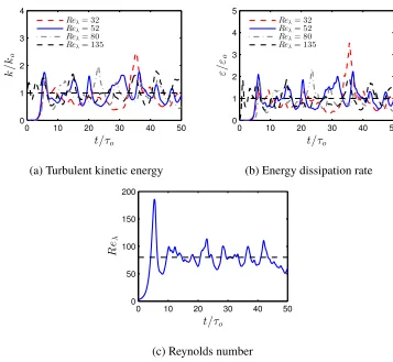
Figure 2.3: a) Turbulent kinetic energy normalized by its expected value (Eq. 2.39). b) Energy dissipation rate normalized by its expected value (Eq. 2.40). c) Taylor microscale Reynolds number,Reλ, for DNS 3. Dashed line corresponds toReo_λ = 80.

The initial velocity fields are generated randomly, using the method suggested by Eswaran and Pope [28]. These velocity fields conform to a specified Passot-Pouquet energy spectrum [60] and are divergence free, as is required for constant density flows.

Multiple simulations are performed at different expected values ofReλ. The simu-lation parameters for the four different cases are tabulated in Table 2.1. Cases 1 and 2 were performed to investigate low Reynolds number effects, if any. Cases 3 and 4 are chosen so the Reynolds number is comparable to simulations and experiments, published in literature (See Table 2.3 for a full list of experimental and full domain DNS studies). More precisely, case 3 has a similar Reynolds number to cases 1 [70], 4 [86] and 8 [10] from Table 2.3; case 4 has a Reynolds number close to cases 5 [35] and 9 [88] in Table 2.3.

(44)

Table 2.2: Results from shear turbulence simulations in triply periodic cubic simu-lations

No Re_λo Reλ u0x/urms u0y/urms u0z/urms hu0xu0yi/k `/L

1 36 32±6 1.26 0.90 0.77 0.42 0.24

2 54 52±9 1.23 0.93 0.78 0.41 0.27

3 80 80±13 1.23 0.92 0.78 0.39 0.28

3a 80 80±15 1.21 0.94 0.79 0.39 0.27

3b 80 80±13 1.20 0.95 0.80 0.38 0.26

3c 80 121±20 1.23 0.93 0.79 0.37

-3d 80 85±10 1.23 0.94 0.78 0.39 0.29

4 128 135±23 1.22 0.93 0.80 0.38 0.31

the simulations were stable. The average values for the numerical results were calculated in the range, 10τoto 50τo.

2.4.2 Temporal evolution

Since the configuration is periodic in all three directions, and spatially homogeneous, ensemble averaged mean quantities are calculated as spatial averages (h · i). These spatial averages are plotted as a function of time.

The time evolution of the integral length scale is plotted in Fig. 2.2a, and after an initial transient period of at most 10τo gives a mean value of about 0.28L, which is slightly higher than the 0.2L for isotropic turbulence observed by Rosales and Meneveau [72]. The integral length scale reaching a statistically stationary value of the order of the domain width is consistent with past simulations of statistically stationary homogeneous shear turbulence [81].

Since the largest gradient of the mean flow is the shear strain ∂ux

∂y, the only significant Reynolds stress term is hu0xu0yi. This is reflected by the simulation, as the forcing term is in the equation for the axial velocity(u0x), proportional to the cross-stream

velocity(u0_y). So, it is expected thatu0xandu0yhave a significant positive correlation. This is one of the major differences between HIT and HST, as there is no correlation among the velocities in different directions for the isotropic case. Figure 2.2b shows thehu0_xu0_yivalues normalized byk at differentReλ. It can be seen that after 5τo, the values fluctuate around 0.4 for all cases, in good agreement with each other.