Optomechanics with Superfluid Helium 4

(1)

Optomechanics with Superfluid Helium-4

Thesis by

Laura De Lorenzo

In Partial Fulfillment of the Requirements

for the Degree of

Doctor of Philosophy

California Institute of Technology

Pasadena, California

2016

(2)

c

2016

Laura De Lorenzo

(3)

To John

”Deep into that darkness peering, long I stood there wondering, fearing,

(4)

Acknowledgements

There are many people to whom I owe my gratitude for their guidance and support along

this journey. Firstly I would like to thank my adviser, Professor Keith Schwab, for teaching

me how to approach a new and challenging experiment and for mentorship and counsel

throughout my PhD. I would like to acknowledge the other members of my thesis and

candidacy committees: Professor Rana Adhikari, Professor Yanbei Chen, Professor Andrei

Faraon and Professor Kerry Vahala. Thank you for lending your time and expertise.

It is my pleasure to recognize all my fellow graduate students and the post docs whose

time in the Schwab lab overlapped with mine: Ari Weinstein, Chan U Lei, Emma Wollman,

Junho Suh, KC Fong, Matt Shaw, Harish Ravi, Harpreet Arora, and Aaron Pearlman. Thank

you for your advice and support. I wouldn’t have made it through without you. I would also

like to thank our theory collaborators, Swati Singh and Igor Pikovski, for patiently teaching

me about gravitational wave detectors. I would be remiss if I did not also recognize the

members of the Eisenstein lab, specifically Debaleena Nandi, Chandni U., Erik Henriksen,

and Johannes Pollanen. Thank you for countless discussions and encouragement and for

the use of your vacuum furnace. I must also thank Tim Blasius and Louise Reina for being

supportive and understanding friends. Thank you to the many other graduate students

and post docs who encouraged me along the way: Alex Krause, Richard Norte, Simon

Gr¨oblacher, Carly Donahue, Justin Cohen, Se´an Meenehan, Jeff Hill, Amir Safavi-Naeini,

and Tao Paraiso.

I would like to recognize support from Mark and Bo in the PMA machine shop. Thank

you for teaching me how to use the lathe and the mill and for hours of machining advice and

(5)

It is my pleasure to recognize my friends Eisha, Christy, and Jim for being my workout

buddies and for bringing some outside perspective to my life. Most importantly, I would like

to express my gratitude to my family: my parents, my brother Donald, sister-in-law Jen, and

my sister Julie. Certainly I would not be here today without you. Finally, I am indebted to

(6)

Abstract

We demonstrate the utility of superfluid helium-4 as an extremely low loss optomechanical

element. We form an optomechanical system with a cylindrical niobium superconducting

TE011 resonator whose 40 cm3 inner cylindrical cavity is filled with 4He. [1] Coupling is

realized via the variations in permittivity resulting from the density profile of the acoustic

modes. Acoustic losses in helium-4 below 500 mK are governed by the intrinsic nonlinearity

of sound, leading to an attenuation which drops as T4, indicating the possibility of quality factors (Q) over 1010 _{at 10 mK. In our lowest loss mode, we demonstrate this}_T4 _{law down to}

50 mK, realizing an acoustic Q of 1.35·108 at 8.1 kHz. When coupled with a low phase noise microwave source, we expect this system to be utilized as a probe of macroscopic quantized

motion, for precision measurements to search for fundamental physical length scales, and as

a continuous gravitational wave detector. Our estimates suggest that a resonant superfluid

acoustic system could exceed the sensitivity of current broad-band detectors for narrow-band

(7)

List of Figures

1.1 The heat capacity of helium versus temperature. The transition point at 2.17

K is known as Tλ because of the shape of the heat capacity through transition. 6

1.2 a) The dispersion curve of helium II showing the linear phonon contribution

(blue) and the roton minimum (red). b) The superfluid (red) and normal fluid

(blue) fractions of helium below Tλ . . . 10

2.1 a) An SEM of a nanomechanical resonator used in our lab, showing a capacitor

with the top plate suspended surrounded by a spiral inductor (courtesy Chan

U Lei). b) The canonical example of a microwave optomechanical system: an

RLC circuit with a capacitor plate that is free to vibrate. . . 15

2.2 Diagrams of our superfluid optomechanical systems: a) the cylindrical niobium

cell with an inner diameter of 3.56 cm and height of 3.95 cm. Two hermetically

sealed dielectric probes are used to couple microwaves into and out of the cavity.

A capillary allows the cell to be filled at low temperatures. b) A vertical slice

through the center of the sapphire cavity setup, showing the ring of 4He and

the fill line. The top cylinder, which supports the whispering gallery modes,

is 5 cm in diameter and 3.1 cm in height. The helium annulus has an inner

diameter of 2.2 cm, an outer diameter of 4 cm, and a height of 0.64 cm. The

sapphire and the microwave couplers are mounted to an aluminum cavity which

reduces the microwave loss from the evanescent fields. . . 17

(12)

2.4 The profiles of every superfluid acoustic mode for the niobium cavity design up

to a frequency of 12 kHz. Below each mode is its frequency and mode number

(l, m, n), where l, m, and n indicate the number of nodes in the longitudinal, azimuthal, and radial directions. The white areas of the profiles indicate node

locations. . . 32

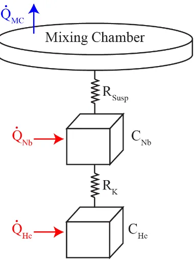
2.5 A simplified representation of the thermal conduction from the superfluid

he-lium to the mixing chamber. The helium is treated as a capacitance CHe

connected to the cell CN b through the Kapitza boundary resistance RK, and

the cell is connected to the mixing chamber through the resistance of the

sus-pension system RSusp. Arrows represent heating due to dielectric loss in both

the niobium ( ˙QN b) and the helium ( ˙QHe) and the cooling power of the dilution

refrigerator ( ˙QM C). . . 40

2.6 The maximum temperature increase (red) and decrease (blue) over which a

source originally centered in the superfluid acoustic resonator will remain within

the bandwidth of the resonator, assuming that at all temperatures the Q is limited by the three phonon process. . . 43

3.1 The equivalent circuit model for the inductively coupled niobium cavity (RC, LC, CC)

parametrically coupled to the superfluid acoustic mode (CM). . . 45

3.2 a) The input circuit inductively coupled to the microwave cavity and b) its T

circuit equivalent. . . 47

3.3 The Thevenin (series) and Norton (parallel) equivalent circuits. The impedance

Zth =ZN. . . 48

3.4 Solving for the thevenin impedance (Zth) of Fig. (3.2b). The intermediate

impedances Z1 and Z2 are referenced in the text. . . 49 3.5 The parallel equivalent to Fig. (3.1). On the right the simplified version where

the resistors Rext andRC are combined into RT and the capacitors CC andCM

(13)

3.6 The scattering picture for a cavity drive tone (ωp) applied on either the red

or blue sideband. On the red or Anti-Stokes sideband, the pump frequency is

ωp = ωC −ωM and the upper sideband is incident with ωC; in this case the

mechanics is preferentially damped. For a drive on the blue or Stokes sideband

the pump frequency is ωp =ωC +ωM, the lower sideband is incident with ωC,

and the mechanics is driven to higher occupations. . . 65

3.7 The phonon occupation of the mechanical mode is determined by its coupling

both to the thermal bath through its intrinsic dissipationγM and to the optical

bath through the optomechanical coupling rate Γopt. . . 68

4.1 Possible a)four phonon and b)three phonon scattering processes. . . 72

4.2 shows the expected absorption coefficient for an 8.1 kHz mode from the 3PP

(green) and the 3_{He impurity for concentrations} _x _{=: 10}−7 _{(red), 10}−9 _(blue),

10−10 _{(black), and 10}−12 _{(grey), assuming the mean free path of} 3_{He atoms}

becomes limited by the cell diameter of 3.6 cm. . . 75

4.3 shows the expected quality factor versus temperature for an 8.1 kHz mode

including effects of both the 3PP and the3_{He impurity for concentrations} _x_=:

10−7 _{(red), 10}−9 _{(blue), 10}−10 _{(black), and 10}−12 _{(grey), assuming the mean}

free path of 3_{He atoms becomes limited by the cell diameter of 3.6 cm. . . . .} ₇₈

4.4 A simplified diagram of how helium-4 can be isotopically purified via heat flush.

The helium-3 atoms move with the normal fluid component. In the counterflow

that is set up when helium II is heated, the normal fluid flows away from the

heat source while the superfluid flows toward it. The superleak serves to define

the direction with which the normal fluid moves away from the resistor. . . 81

4.5 COMSOL simulation showing distortions of the niobium cell due to the l = 1,

m = 0, n= 0 superfluid acoustic mode with a frequency of 5984 Hz. . . 86 5.1 Pictures of the niobium microwave cavity after etching, showing a mirror finish:

(14)

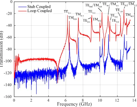
5.2 Transmission spectrum of the niobium cavity at 300K for stub couplers (blue)

and loop couplers (red). In both the loop and stub coupled cavities, the couplers

are located on the lid at a radius r = 0.64a (a is the cavity radius), where the TE011 magnetic mode is maximum. Modes are labeled by TE or TM and the

mode number (n,m,l). There are three sets of degenerate modes: TE010/TM110,

TE011/TM111 and TE012/TM112. . . 94

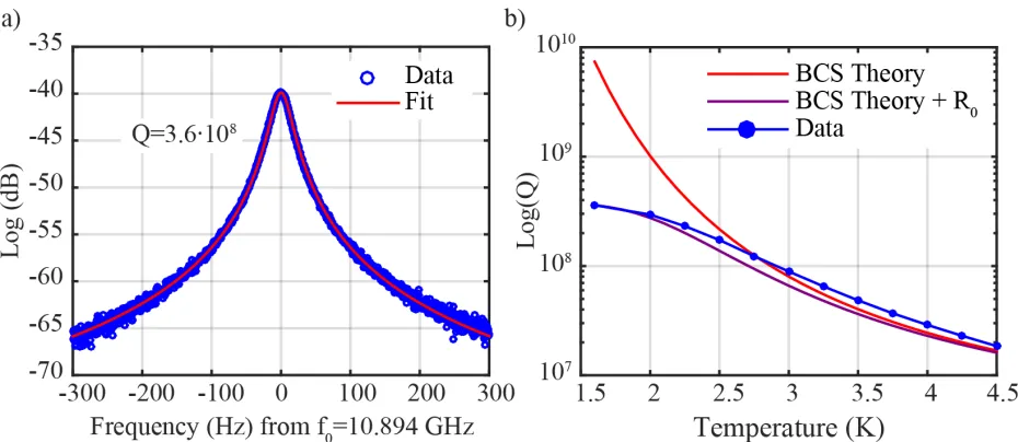
5.3 (a) S21 measurement of the TE011 mode at 1.6 K, demonstrating a microwave

Q of 3.60·108 _{or a cavity linewidth of 30 Hz. (b)}_Q _{of the TE}

011 mode versus

temperature. Data is represented by blue circles and the connecting line is a

guide to the eye only. The red line is the expected quality factor from the BCS

losses of Eqn. (2.20). The purple line is the expected quality factor including

both the BCS loss and the residual resistance R0, where R0 is calculated from

the highest Q data point and found to be 2 µΩ. . . 96 5.4 The plumping panel used to fill the niobium cavity with helium. . . 97

5.5 The helium fill line from the 1 K plate to the niobium cell. The line is thermally

anchored at each stage with sintered-silver heat exchangers. . . 99

5.6 The plumbing panel used to actuate the cryogenic valve. . . 102

5.7 From Run 4, January 2015: a) With the cell on the fridge and initially under

vacuum, frequency shifts of the TE011 mode while filling the cell with4He gas.

The cell is filled by applying ≈ 1.2 bar of pressure from the helium cylinder attached to the plumbing panel. Notice the impedance of the fill line is such that

filling requires ≈30 minutes. b) With the cell on the fridge and initially filled

with about one bar of 4He gas, frequency shifts of the cell while evacuating

to vacuum. After 90 minutes of pumping, the cell’s frequency has returned

approximately to the starting vacuum frequency from a). An additional 30

minutes or even 130 minutes of pumping do not appear to shift the frequency

(15)

5.8 From Run 4, January 2015: The TE011 and TM111 modes at 77 K. Notice that

the TE011 appears as a dip rather than a peak. Checking the frequency shifts

is easier using the TM111 mode in this case. . . 107

5.9 From Run 4, January 2015: a) Frequency shifts of the TM111 mode as the cell is

filled with4_{He gas, starting with the cell in vacuum and thermalized to}_≈_{77 K.}

Notice that the total frequency shift is greater than at 300 K because helium is

denser at lower temperatures. Also note that the frequency shifts more quickly

because the conductance of capillaries improves at lower temperatures as the

background pressure drops. b) Pumping on the cell at 77K with the cryogenic

valve closed. The TM111 mode frequency remains constant as expected if no

helium is exiting the cell. c) Pumping on the cell at 77K with the cryogenic

valve open. The frequency shifts back to the vacuum value within about an

hour. . . 109

5.10 a) The vapor pressure of helium versus temperature and b) the density of helium

versus temperature. . . 111

5.11 Pictures of the cell for each run of the fridge with complete descriptions given

in the text: a) Run 1, b) Run 2, c) Run 3, d) Run 4, and e) Run 5. . . 112

5.12 A schematic of the microwave measurement circuit. OS2 is a microwave signal

generator used to pump the niobium cavity on the red sideband (ωp =ωC−ωM).

OS1 is an audio frequency generator used to drive the piezoelectric actuator

(PZT) which excites the acoustic mode. The upconverted signal from the

su-perfluid acoustic mode is mixed down to an audio signal and measured on a

lock-in amplifier. . . 113

5.13 Superfliud acoustic Q versus mixing chamber temperature for the first run (circles) and second run (triangles) of the experiment. Each color denotes a

different mode, as shown in the legend. The red line shows the expected loss

from the 3PP (Eqn. (4.2)) and the blue line shows the expected loss from the

(16)

5.14 The frequency of the TE011 mode at 550 mK before and after the 3 Vpp piezo

drive for the 10 kHz mode is turned on. Notice that, before the drive, the

frequency is stable (the 10 and 20 minute plots are on top of each other), but

after the drive is turned on, the mode shifts up in frequency until it reaches a

new stable value (the 50 and 60 min plots are on top of each other). The new

value is about 1 kHz above the original frequency, or ≈3 cavity linewidths. . . 123

5.15 Superfliud acoustic Q versus mixing chamber temperature for the third run

(circles) and fourth run (triangles) of the experiment. Each color denotes a

from the 3PP (Eqn. (4.2)), while the navy blue and light blue lines show the

dissipation expected from3He impurities at concentrations of 10−6 (Eqn. (4.5))

and 2·10−10 _{(Eqn. (4.6)), respectively, assuming in all cases a mode frequency}

of 8115 Hz. . . 125

5.16 The frequency of the TE011 mode with the cell full of helium, cryogenic valve

closed, and fridge at its base temperature while the fill line from the cryogenic

valve to room temperature was evacuated with a rough pump. Notice that

the cell frequency continued to shift upward indicating that the cell was slowly

emptying and the cryogenic valve was not leak tight to superfluid 4_{He. . . 127}

5.17 The continuous heat exchanger of our Kelvinox 400H dilution refrigerator with

Teflon shims inserted between each coil at 90 degree increments. . . 128

5.18 A ring down of the 8115 Hz mode, showing the highest quality factor we have

measured: 1.35·108_{. The mixing chamber temperature was 30 mK, but if the}

(17)

5.19 Thermalization curves for the superfluid helium, extracted from the quality

factor of the 8115 Hz mode by assumingQis limited by the 3PP, upon heating the fridge to a) 50 mK, b) 60 mK, c) 80 mK, and d) 200 mK. Data points

are shown as red circles; the black line is an exponential fit to the data. The

final fridge temperature and the time constant of the exponential fit are shown

on each figure. Notice that the final temperature of the helium in some cases

differs from the mixing chamber temperature. . . 130

5.20 The thermal time constants calculated from the exponential fits in Fig. (5.19)

plotted versus the final fridge temperature for each data set. The connecting

line serves as a guide to the eye only. Notice that the time constants at low

temperatures are extremely long. . . 131

5.21 Superfliud acoustic Q versus mixing chamber temperature. Data from Run 5

are shown as diamonds at 20 mK. For comparison the data from Runs 3 and

4 are shown as faded circles and triangles, respectively. Each color denotes a

from the 3PP (Eqn. (4.2)), while the navy blue and light blue lines show the

dissipation expected from3He impurities at concentrations of 10−6 (Eqn. (4.5))

and 2·10−10 _{(Eqn. (4.6)), respectively, assuming in all cases a mode frequency}

of 8115 Hz. . . 134

5.22 Helium temperature inferred from the measured superfluid acoustic quality

factor versus power incident on the cavity. The blue and red lines indicate that

the cell is attached to the mixing chamber with a copper wire (Run 4) or a

silver rod (Run 5), respectively. Note that while the heating is reduced with

(18)

5.23 a) the Pound Drever Hall frequency stabilization circuit. AM modulation is

used to add sidebands to the source before it is incident on the cavity. The

signal from the cavity is split in two: one branch is measured on a spectrum

analyzer (SA) and the second is mixed down to the sideband frequency and

measured on a lock-in. One quadrature of the signal from the transmitted

sidebands is used as an error signal, which is first fed into a PID controller and

then input to the FM modulation on the source. The red circuit is at acoustic

frequencies and the blue circuit is the error signal. b) the PDH error signal

from the lock-in. . . 138

5.24 Pictures of the cell planned for future runs: a) is similar to the copper wire

setup used in Runs 3 and 4, but with an annealed 5N silver wire with a diameter

of 0.10 cm. The copper tubes to which the wire is soldered are machined with a smaller diameter section at the top (0.635 cm) so that the wire exits closer to the cell’s center keeping the cell level. b) shows a different approach to

attaching the wire to the the cell and fridge. One copper piece is bolted to

cell (or fridge), and a second copper piece is used to clamp onto the 0.23 cm diameter silver wire. . . 139

5.25 Damage to the niobium lid preventing leak tight operation of the cell . . . 140

5.26 Pictures of machined valve pieces for design 2. The housing is brass, the guide,

plunger, and seal are stainless steel, the needle is Torlon, and the bellows are

nickel. Here the bellows have already been soldered to the plunger and guide. 144

5.27 The sapphire pieces after machining: a) the bottom piece of the cavity design,

showing the annular cavity that will be filled with helium, b) the top piece of

the cavity design, c) the test piece of equal size to the final bonded piece, before

(19)

5.28 The bonded and polished sapphire cavity: a) side view. Note the discontinuity

in the outer edge at the location of the bond line, b) top view, c) view from the

top edge with the cavity sitting in the base of the aluminum shielding cavity.

Notice the fill line connecting the annular cavity to the base of the sapphire

mushroom. . . 147

5.29 a) Transmission measurements of the highest Qmode of the test resonator (no annular cavity) at both 300K (red, f0 = 10.97 GHz) and 77K (blue, f0 = 11.06

GHz). At 300 K, the Q is 66·103_{, and at 77 K the} _Q_{s of the left and right}

peaks are 2.4·106 and 2.8· 106, respectively. b) The highest quality factor ”mode” that could be found at 77K in the spectrum of the bonded resonator,

f0 = 11.05 GHz. . . 148

6.1 The phonon occupation of the superfluid acoustic mode versus the number of

pump photons (nP) in the sideband cooling tone, ignoring the effects of

dielec-tric heating, for three starting temperatures: 40 (blue), 20 (green) and 10 mK

(red), assuming that Qis limited by temperature. In each case, the curve that continues to drop with increasing photon number ignores the effect of source

phase noise, while the curve that reaches a local minimum includes the effect.

The black curves denote sources of various phase noise (−140,−160,−180,−200 dBc/Hz), as labeled on the figure. . . 150

6.2 The phonon occupation of the superfluid acoustic mode versus the number

of pump photons (nP) in the sideband cooling tone, including the effects of

dielectric heating, for three starting temperatures: 40 (blue), 20 (green) and 10

mK (red), assuming that Q is limited by temperature. In each case, the curve that continues to drop with increasing photon number ignores the effects of

heating and source phase noise, while the curve that reaches a local minimum

includes both effects. The black curves denote sources of various phase noise

(20)

6.3 A schematic of our low phase noise microwave source as described in the text.

The left circuit is the self resonant loop of a sapphire whispering gallery mode

resonator, with control loops for both phase (red) and amplitude (blue). The

right circuit consists of a microwave source and a divider and provides tunability

to the source. . . 153

6.4 The minimum detectable strainhmin versus integration timeτint for our

super-fliud acoustic detectors [2], G1 (blue) and G2 (red) assuming mechanical Q of

1010 _{(dotted) and 10}11 _{(solid). Also shown is the achieved strain sensitivity of}

LIGO-S6 (solid, black) and the design sensitivity of advanced LIGO (dotted

black). The stars indicate the limit set by LIGO and the limit expected from

advanced LIGO. The spin down limit of the pulsar J1301+0833 is also shown

as the dotted horizontal line. . . 159

6.5 The experimental scheme proposed by Pikovski et al. [3] to measure the

commu-tator’s deformation. An input signal is incident on a polarizing beam splitter,

then an electro optic modulator and a second beam splitter. The field reflects

from the optical cavity and enters the delay line. The length of the delay line is

such that the mechanical oscillator evolves by one quarter of a mechanical

pe-riod between each interaction. After all four interactions, the signal is measured

interforemetrically with the reference. . . 162

6.6 The minimum required pump power to achievenM << λNP. The red line shows

nM/λresulting from the sideband cooling tone with pump photonsnP. nP from

the sideband cooling tone is shown with the green line. The blue line shows

the total of nP from the sideband cooling tone plus NP =nm/λ·10 (fulfilling

NP >> nm/λ) for the phase space manipulations of Pikovski et al.’s [3] scheme. 164

(21)

C.2 Drawing of the cylinder top, machined from niobium with a minimum purity

of 99.8%. Shown here is the final design with the fill line and microwave ports

located at the position of the radial node in helium modes with only one radial

node. . . 172

C.3 Drawings of the cap for the microwave ports of niobium cavity. Shown is the final design with cutouts to allow all the pieces to fit on the niobium cavity lid. 173 D.1 Drawing of the valve assembly. . . 174

D.2 Drawing of the guide, which is made from stainless steel. . . 175

D.3 Drawing of the housing, which is made from brass. . . 176

D.4 Drawing of the seal, which is made from stainless steel. . . 177

D.5 Drawing of the plunger, which is made from stainless steel. . . 178

D.6 Drawing of the needle, which is made from Torlon, a stiff plastic that does not easily deform at low temperatures. . . 179

E.1 Drawing of the top for the sintered-silver heat exchangers. . . 180

E.2 Drawing of the bottom for the sintered-silver heat exchangers. . . 181

E.3 Drawing of the sintered-silver heat exchangers assembly. . . 182

E.4 Drawing of the pressing piece for the sintered-silver heat exchangers. . . 183

F.1 Drawing of the copper L brackets used to mount the cell to the mixing chamber in Run 1. . . 184

F.2 Drawing of the square copper bracket used to mount the cell to the mixing chamber in Run 2. . . 185

F.3 Drawing of the silver rod used to mount the cell to the mixing chamber in Run 5.186 G.1 Drawing of the sapphire test resonator. . . 187

G.2 Drawing of the bottom sapphire piece for the two piece helium filled sapphire cavity. . . 188

(22)

List of Tables

4.1 The highest measured mechanical quality factors of several high Q materials. Also shown are the frequency of the measure mode and the temperature at

which the measurement was taken. . . 85

5.1 The TE and TM mode frequencies up to 13.5 GHz for the niobium cavity. The

expected frequencies are calculated from Eqns. (5.1) and (5.2) for a cavity

with a diameter of 3.556 cm and length of 3.955 cm. The frequencies were

measured with a vector network analyzer at 300 K and the spectrum is given

by the red line shown in Fig. (5.2). The final column shows the difference

between expected and measured frequencies: (fexp−fmeas)/fexp · 100. The

only experimentally missing modes are the TE110, TE210, and TE310. . . 95

5.2 A table of the superfluid acoustic modes up to and including the highest

fre-quency mode found experimentally. The first column gives the mode numbers,

the second the expected frequency from Eqn. (2.24). The third column

indi-cates whether or not the mode is degenerate. The fourth column is the

experi-mentally measured frequency of the mode from Run 4 at the base temperature

of fridge; for most of the degenerate modes, only one peak could be found, and

many modes were altogether not detectable. The fifth column is the highest Q

(23)

5.3 Table describing the approximate diameter (d) inµm and length (L) in m of the fill line between the 1 K plate, still, cold plate (CP), mixing chamber (MC), and

cell for each run of the experiment. Not shown is the capillary connecting the

room temperature valve at the top of the fridge to the 1 K stage, which is 300

µm in diameter and≈1.3 m in length; this line was provided by Oxford and has remained unaltered. Over time, the capillaries below 1 K have been increased

in length and decreased in diameter in order to limit thermal conduction and

acoustic losses. . . 117

5.4 Table summarizing the changes in the experimental setup for all fridge runs,

including the choice of cavity suspension, the final coaxial cabling to the cell,

and other important notes. . . 117

A.1 Table of variables . . . 167

B.1 Bessel function zeros. . . 168

B.2 Bessel function extrema, microwave modes. . . 169

(24)

Chapter 1 Helium-4

1.1 Historic Background

Helium is an element of superlatives: along with neon, it is the only element for which no

known compounds exist; additionally, it is the lone element which does not freeze without

pressurization. After hydrogen, helium is both the second lightest and second most abundant

element, comprising 24% of the universe’s elemental mass [4]. Because of its unique

proper-ties, helium played a central role in refrigeration techniques and in low temperature physics,

enabling such monumental discoveries as superconductivity and superfluidity [5]. Today

liq-uid4_{He has widespread use as a coolant for superconducting magnets with applications from}

MRI machines to the Large Hadron Collider. Further, the invention of the dilution

refrig-erator, a continuously running cryostat which relies on the dilution of the lighter isotope

3_{He with the significantly more common} 4_{He, eventually led to a commercial product which}

reliably reaches temperatures in the tens of millikelvin range. The dilution refrigerator has

become an indispensable tool in physics, in fields as varied as quantum information and

fundamental studies of condensed matter. Since the existence of helium was confirmed in

1895, few elements have had the the same tremendous impact on physics.

The first hints of helium’s discovery came in August of 1868, when French astronomer

Pierre-Jules-C´esar Janssen observed a new spectral line in the sun’s prominence during a

solar eclipse in India [6]. Because of its proximity to the sodium doublet, this line was

(25)

the same 587.49 nm yellow line in October of 1868, while observing the prominence in

London [4]. At the time, neither man accorded D3 much significance, other than to report

its existence. Both Janssen and Lockyer were recognized instead for independently arriving

at a new spectroscopic method, which allowed viewing of the prominence of the sun in the

absence of an eclipse [6].

Lockyer did however continue to study the sun, teaming with noted British chemist

Edward Frankland to outline the composition of the prominences by reproducing spectral

observations with known gases in a laboratory setting. While it was only a small piece of their

work, Lockyer and Frankland tried recreating D3 with hydrogen at various temperatures and

pressures [6]. After failing to do so, they began informally referring to the line as ”helium,”

without any public claim of discovery. The name derives from the Greek word ”helios,” for

sun, and the ending ”ium” reflected their belief that a metallic element was responsible for

D3 [4]. The word ”helium” does not appear in literature until 1871, when president of the

British Association for the Advancement of Science, William Thomson, noted that Frankland

and Lockyer proposed that an as yet unknown substance produced the D3 spectral line [6].

The claim was met critically by the scientific community at the time, as a mere spectral

observation failed to meet the standard of elemental discovery. Notably, Mendeleev, who

was responsible for creating the periodic table of the elements, publicly noted that such an

assumption was unjustified in 1889 [6].

While there was no consensus of ”helium’s” existence, it was known widely in literature,

though often referred to simply as the ”D3 spectral line.” It was at first thought to occur

only in the sun but was later found in many other stars throughout the universe. In fact,

helium is one of the most common elements in stars, where it is formed from nuclear fusion

of hydrogen atoms [4]. In 1882, Italian geologist Luigi Palmieri claimed to find the D3 line

in gases escaping from a volcanic eruption at Mt. Vesuvius [6]. However he failed to collect

any of the gas and his claim remained unsubstantiated. Helium was also mentioned by many

scientists who thought it was a constituent form of matter. For example, British chemist

William Crookes theorized that due to its light weight, as evidenced by its presence in the

(26)

In 1889 American geochemist William Francis Hillebrand was studying samples of the

mineral uraninite (UO2) when he noted bubbling from the material after exposure to

sul-phuric acid. He collected and analyzed the gas, determining it to be nitrogen [6]. On a hunch

informed by Hillebrand’s work, in 1895 William Ramsay obtained a sample of clevite

(urani-nite with about 10% other rare minerals), to look for compounds of the newly discovered

gas argon. He quickly realized he had discovered a new gas that was neither nitrogen nor

argon, and upon observation of the telltale D3 spectral line, he concluded that this at last

was the elusive helium [6]. Working independently, Per Theodor Cleve and his student Nils

Abraham Langlet also discovered helium in samples of clevite in Uppsala, Sweden. Langlet

was further able to measure helium’s density to be twice that of hydrogen [6].

Interestingly, in April of 1895, Ramsay wrote to Lockyer suggesting a name change to

”helion” in keeping with the other noble gases, but nothing came of his request [4].

Even after helium’s discovery in uranium minerals, it was thought to be extraordinarily

rare on Earth. Because of the helium atom’s small mass, it moves with velocities fast

enough to escape the Earth’s gravitational pull. While helium would have been a dominant

component of Earth’s early atmosphere, today it comprises only 0.00052%. Though helium

was discovered in uranium minerals, it exists there only in trace amounts.

The assumption of helium’s scarcity changed in 1903, when a company drilling for natural

gas near Dexter, Kansas struck a geyser of gas, escaping at a rate of 9 million cubic feet

per day [7]. To celebrate their find and the expectant economic boom for the town, the

people of Dexter planned to light the gas on fire using a burning bale of hay. After a day

of jubilation, the hay bale failed to light the geyser. In fact, the flame was extinguished on

repeated trials [7]. Intrigued, geologist Erasmus Howard collected samples of the gas and

analyzed them at the University of Kansas. With the help of colleagues Hamily Cady and

David McFarland, the mysterious gas was determined to be only 15 % methane and 72%

nitrogen. Most interestingly, after using charcoal immersed in liquid air to remove the other

components, they found the signature D3 spectral line and determined the gas was almost

2% helium [7]. To this day, natural gas fields, where it is a product of radioactive alpha

(27)

Soon after helium’s discovery on Earth, there was a race to liquefy the newfound

ele-ment. Heike Kamerlingh Onnes of Leiden became the first to do so in 1908, using Joules

Thompson cooling. He found that helium-4 liquified at 4.2 Kelvin. Onnes’ work opened up

new frontiers in cryogenic physics, paving the way for important discoveries. Most notably,

superconductivity was discovered only three years later, in 1911; today Onnes is known as

”the father of low-temperature physics [5].”

1.2 Basic Properties

The most common isotope of helium is helium-4, which is composed of two protons and two

neutrons. Having no nuclear spin, 4_{He behaves as a boson. The only other stable isotope}

is helium-3, which has a fractional abundance of about 1 part in 106 [8]. With only one

neutron, 3_{He is a fermion and thus behaves very differently from helium-4. Though neither}

are stable, two other helium isotopes have been observed: helium-6, which has a half life

τ1/2 = 0.82 s and helium-8, with a half life ofτ1/2 = 0.12 s [4].

With two electrons, helium has a filled s shell, resulting in a highly symmetric structure.

The sole permanent dipole exists in the isotope3_{He, which has a small nuclear magnetic}

mo-ment. For helium-4, the only interatomic binding force is the attractive interaction between

momentarily induced dipoles known as the van der Waals force. Further, the van der Waals

force between helium atoms is the weakest of any substance. The weak interatomic forces

coupled with the small atomic masses lead to low boiling temperatures of 4.21 K (helium-4)

and 3.19 K (helium-3); these are the lowest boiling points of all known substances.

As mentioned above, solidifying helium cannot be done with temperature alone; it

re-quires 25 bar of pressure. Imagine that each atom occupies a volume of space, roughly a

sphere of radius R = V_A1/3 where VA is the atomic volume. From quantum mechanics we

(28)

each atom has an energy of localization given by [9]:

E0 ≈(δp) 2

/2m4 =

h2

2m4V 2/3

A

, (1.1)

where m4 is the mass of a helium-4 atom. Because of helium’s small mass, the zero point

energy is comparable in magnitude to the potential energy of the liquid state. Therefore

the total energy of the liquid state reaches a minimum at a high atomic volume. While at

low enough temperatures (T <4.2 K), the interatomic potentials become strong enough to form a liquid, the liquid state remains low density, and the solid state does not form with

temperature alone.

1.3 Two Fluid Model

As liquid helium is cooled beyond 4.2 K it undergoes a second order phase transition at a

critical temperatureTλ = 2.17 K. This temperature is known as the lambda point because of

the shape of the specific heat versus temperature through transition (see Fig. (1.1)). Below

(29)

[image:29.612.75.539.74.379.2]

Figure 1.1: The heat capacity of helium versus temperature. The transition point at 2.17 K is known asTλ

because of the shape of the heat capacity through transition.

One of the interesting and initially unexplained results from early experiments on HeII

was the measurement dependent viscosity of the fluid. Measurements of rotating viscometers

showed a resistance not much different from that of 4He gas. Meanwhile, measurements

of viscosity based on flow rates through small capillaries demonstrated flow rates nearly

independent of the pressure differential, indicating virtually zero resistance to flow.

Tisza [10] was able to reconcile these results with the two fluid model of helium-4: below

Tλ, helium behaves as if it were composed of two non interacting fluids, which are called

the superfluid and the normal fluid. The total density of helium (ρ) can be written as the combination [11]:

ρ=ρN +ρS, (1.2)

(30)

relative values of the densities depend on temperature; At absolute zero,ρN = 0 andρS =ρ

while at Tλ,ρN =ρ and ρS = 0.

The superfluid component moves without viscosity and carries no entropy. It is the

superfluid component which can flow without friction through a small capillary. The normal

fluid component behaves like an ordinary viscous liquid and carries the total entropy of the

fluid. Andronikashvili’s experiment, where he measured the fluid’s viscosity with a rotating

wire viscometer, famously produced a curve of normal fluid density versus temperature [12];

see Fig. (1.2b).

While the two fluid model has been very successful in explaining the experimental

be-havior of helium-4, it is important to remember that all helium atoms are identical. It is not

possible to pick an individual atom and claim that it is part of the superfluid or the normal

fluid component.

1.4 Equations of Motion

We will now enumerate the equations of motion for HeII. Each fluid moves with its own local

velocity so the total momentum per unit volume can be written as [11]:

j=ρNvN+ρSvS, (1.3)

where vN and vS denote the velocities of the normal fluid and superfluid components. The

momentum is related to the density (ρ) through the equation of continuity:

∇ ·j=−∂ρ

∂t. (1.4)

Euler’s equation of motion in the absence of viscosity and for small velocities, where quadratic

terms in the velocity can be discarded, gives [11]:

∂j

(31)

whereP is the pressure. When viscosity can be ignored, the fluid motions are reversible and entropy is conserved. In this limit [11]:

∂(ρS)

∂t =−∇ ·(ρSvN), (1.6)

where S is the entropy per gram of helium-4. The change in internal energy U of a fluid is given by [11]:

dU =T dS−P dV +GdM, (1.7)

where G is the Gibbs free energy. T is temperature, and dM is a change in the mass. If the mass of the fluid is increased by adding particles to the superfluid, while maintaining

a constant volume, then dV = dS = 0 such that dU = GdM. Therefore the work (W) of moving a mass ∆M of superfluid from point A to point B (dx) is given by:

∆W =∇G·dx·∆M. (1.8)

From this we can write an equation for the motion of the superfluid [11]:

dvS

dt =S∇T −

1

ρ∇P. (1.9)

1.5 Thermomechanical Effect

A classic superfluid helium experiment is the illustration of the fountain effect [13]. A

superleak, formed by packing a tube with emery powder, connects a bath of He II to a small

capillary which emerges from the helium bath. When the capillary side of the superleak is

heated, superfluid flows quickly into the tube and shoots out the end of the capillary like a

fountain.

This simple experiment illustrates the inseparability of mass flow and heat flow in He

II. When the capillary is heated, both its temperature and normal fluid fraction increase

(32)

travel away from the heat source through the superleak; instead, when the capillary is heated,

ρS rushes through the superleak to diminish the superfluid gradient. The superfluid from

the bath flows toward the heat source with enough velocity to form a fountain.

The fountain effect is also known as the thermomechanical effect and we can estimate its

size from the equations of motion. In equilibrium the fluid is not accelerated: dvS/dt = 0.

From Eqn. (1.9) it follows that:

∆P

∆T =ρS. (1.10)

When helium II is heated, normal fluid flows away from the source of heat, and in order to

retain equal density everywhere, the superfluid flows in the opposite direction; this is known

as counterflow. An important implication of this effect is that the fluid emerging from the

capillary is expected to be colder than the bath because its superfluid fraction is greater.

Because3He moves with the normal fluid component, this connection between heat flow and

mass flow can be exploited to isotopically purify 4_{He as will be discussed in Section 4.2.2.}

1.6 Elementary Excitations

Below Tλ, the thermal de Broglie wavelength of the helium atoms becomes comparable to

their interatomic spacing. As noted by Landau [14], at this point the behavior of

super-fluid helium must be described in terms of elementary excitations. These excitations have

energy = c4q, given by the dispersion curve. Here q is momentum and c4 is the speed

of sound. Impressively, Landau deduced a form of the dispersion curve in 1941, which was

not confirmed experimentally until the late 1950s with neutron scattering experiments [11].

It is important to note that in his treatment of helium II, Landau ignored the interactions

between excitations. This is a good approximation at low temperatures where the density

of excitations is small (T < 1.5 K), but as the temperature approaches Tλ this assumption

breaks down and the dispersion curve and helium II properties will be different.

The shape of the helium II dispersion curve is shown in Fig. (1.2a); exact numeric values

(33)

the dispersion curve is linear: =c4q. This region describes the low energy phonons which

move with the sound velocity c4. At higher momenta, the curve reaches a local minimum;

the region around the minimum is specified by:

= ∆ + (q−q0)

2

2µ . (1.11)

From neutron scattering experiments at 1.1 K, these constants are found to be [15]:

∆/kB = 8.65 +/−0.04K,

q0/~= 1.91 +/−0.01 ˚A

−1

, µ= 0.16·m4,

where m4 is the mass of a helium atom, kB = 1.38·10−23 J/K is the Boltzmann constant,

and _~= h/2π = 1.05·10−34 J·s is the reduced Planck constant. The excitations described by this high energy minimum are known as rotons.

Figure 1.2: a) The dispersion curve of helium II showing the linear phonon contribution (blue) and the roton

minimum (red). b) The superfluid (red) and normal fluid (blue) fractions of helium belowTλ

The phonon and roton contributions to the normal fluid density are given by [11]

ρn,ph =

2π2_k4

B

45_~3_c5T 4

(34)

ρn,r =

2µ1/2_q4 0

3 (2π)3/2(kBT)

1/2 ~3

exp−∆/kBT_, _(1.13)

where ∆, q0, and µ are defined as above, by neutron scattering experiments. These two

contributions are equal at ≈ 570 mK; below this temperature the rotons rapidly become

irrelevant. When we consider acoustic loss in 4_{He at dilution refrigerator temperatures, we}

need only consider phonon-phonon collisions because while phonon-roton and roton-roton

collisions will also lead to acoustic loss, the roton population is so small as to make their

contributions irrelevant. At temperatures below about 450 mK, where ρn,r << ρn,ph, we

can write: ρn/ρ≈1.2·10−4T4. We note that helium-4 is unique among the condensates in

that, at experimentally achieved temperatures of T < 10 mK, the fraction of temperature to transistion temperature is T /Tλ < 0.005. In comparison, in 3He, the lowest achieved

temperatures are approximately 200 µK, leading to T /TC < 0.08 [16]. In atomic

Bose-Einstein condensates, the fractional temperature is often T /TC ≈ 0.5 [17]. For helium-4,

this small T /Tλ ratio leads to the incredible conclusion that at 10 mK the non-condensate

fraction is expected to be only ρn/ρ≈10−12.

Finally, we point out that because phonons are the dominant excitation below 570 mK,

we can calculate the specific heat of helium from the Debye theory for solids. One finds that

the specific heat is given by [11]:

CV =

2π2k_B4

15ρ_4~3_c3 4

T3 ≈20.7·T3 J/kg·K. (1.14)

Note thatCV has theT3 dependence that is expected when phonons are responsible for heat

conduction. When we consider the difficulty of cooling our sample to low temperatures, it

will be important that the heat capacity drops rapidly with decreasing temperature.

1.7 Second Sound

Below Tλ, where the two fluid model applies, we expect to find multiple solutions for sound

(35)

above, one can solve for the ordinary longitudinal pressure modes, modulations of density at

constant temperature, which in helium II are known as first sound. Additionally one finds

the relation [11]:

∂2_S

∂x2 =

ρN

ρS

C T S2

∂2_S

∂t2, (1.15)

where C is the heat capacity. (In helium, the heat capacity at constant pressure is nearly equal to the heat capacity at constant volume.) Notice that Eqn. (1.15) is also an equation

for the propagation of sound, but in this case, the waves are variations in entropyS or equiv-alently, temperature T. Because the superfluid component cannot carry entropy, movement of temperature and mass is linked. The normal fluid component carries the entropy while

the superfluid component moves in the opposite direction. These temperature waves are

known as second sound and their velocities can be given by [11]:

c2 =

s

ρST S2

ρNC

. (1.16)

Like first sound, the absorption of second sound in helium II is well studied both theoretically

and experimentally. We introduce second sound because there may be some conversion of

first sound to second sound; given the higher attenuation of second sound this may become

a relevant loss process in very high Q superfluid acoustic resonators.

1.8 Vortices

Finally, we mention that the superfluid can be described by a macroscopic wave function [11]:

ψ =eiPis(Ri)_φ, _(1.17)

where s(Ri) is a function of position and φ corresponds to the ground state at rest. In this

description, the velocity of the fluid depends on the gradient of the phase:

vS(R) = ~

(36)

Consider what happens to a body of liquid helium-4 set into rotation. An ordinary viscous

fluid will rotate as a solid body, but the viscous interactions between atoms are absent in a

superfluid. The condition that∇ ×vS = 0, which is required for the condition of no viscosity

in the superfluid, cannot be universally valid as experiments have shown that helium can be

set into rotation. As suggested by London and Onsager [18] and later found experimentally,

the liquid is permeated by an array of vortex lines which increase the energy but maintain

∇ ×vS = 0 over most of the volume. A vortex line is defined by its circulation κ=

H

v·dl. Vortices can be envisaged as holes in the superfluid helium. Imagine a cylinder submerged

in the fluid; as one moves away from the cylinder a distancer the velocity grows asv =A/r

where A represents a constant. If the cylinder is made small enough, the centrifugal force of the fluid rotation will be strong enough to maintain the hole. The size of the vortex (a0)

can be estimated by balancing the surface tension Tsurf with the Bernoulli force [11]:

a0 =

ρκ2

16π2_T

surf

≈0.3 ˚A. (1.19)

The vortex is a small region of sizea0 where the macroscopic wavefunction tends to zero.

Because 4_{He are bosonic particles, any rotation of the fluid where each atom replaces its}

neighbor produces a state which is indistinguishable from the initial state. Such a rotation

produces a phase change of the macroscopic wave function equal either to zero or an integral

multiple of π. This condition leads to the quantization of circulation: H v·dl = 2π_~n/m

where n is an integer value and m is the mass of a helium atom.

It is not well known how many vortices will be present in a 50 cm3 sample of helium such

as those which we use. There are ways to limit the vortex population, such as by cooling

slowly through the lambda point or by filling a vessel slowly through a sinter. It is also not

known how vortices will interact with first sound and what limitations they may ultimately

(37)

Chapter 2 Optomechanics

2.1 Introduction

Optomechanics is the study of systems with a mechanical mode parametrically coupled to

either a microwave or an optical mode (or both). There are several excellent review papers

outlining both the underlying physics and the experimental results to date; for a recent

review, see Aspelmeyer et al. [19].

The canonical example of a microwave optomechanical system is a parallel RLC circuit

where one of the capacitor plates is free to vibrate; for an illustration, see Fig. (2.1). The

capacitance of a parallel plate capacitor is C =0A/d, where A is the area of the plates and

d the distance between them. As the capacitor plate vibrates, the distance d is modulated, changing both the capacitance of the cavity and its frequency ω = 1/√LC. Exciting a mechanical mode with frequency ωM in the capacitor plate produces sidebands at ωC ±ωM

on the microwave cavity resonance.

The optomechanical Hamiltonian is written as [20]:

H =_~ωC

a†a+ 1 2

+_~ωM

b†b+ 1 2

+g_0~ b†+b

a†a+1 2

, (2.1)

where ωC and ωM are the frequencies of the microwave and mechanical modes and a† (a)

(38)

the frequency of the microwave cavity is pulled by the motion of the mechanics:

g0 =

∂ωC

∂x ∆xZP. (2.2)

g0 depends on the zero point motion ∆xZP which describes the magnitude of the motion of

the mechanical mode in its ground state, where it has a phonon occupation of less than one.

∆xZP depends on the mechanical resonator’s mass m and frequency as:

∆xZP =

r

~

2mωM

. (2.3)

From this definition we note that smaller masses and larger mechanical resonance frequencies

increase the optomechanical coupling rate. As will be elaborated in more detail in Chapter

3, the parametric coupling between the optical and mechanical modes allows one to either

”damp” or ”drive” the mechanics. With high enough coupling rates, the mechanical mode

can be cooled to its ground state, where one expects it may behave quantum mechanically.

Figure 2.1: a) An SEM of a nanomechanical resonator used in our lab, showing a capacitor with the top plate suspended surrounded by a spiral inductor (courtesy Chan U Lei). b) The canonical example of a microwave optomechanical system: an RLC circuit with a capacitor plate that is free to vibrate.

The field of optomechanics spans a wide range in both frequency and mass, from atomic

(39)

understood for decades, recent progress in nanofabrication techniques has permitted the

manufacture of mechanical oscillators with the parameters necessary to achieve ground states

of the mechanics. Ground state cooling was first achieved in 2010 by Andrew Cleland’s lab

at UCSB [22]; this was result was quickly repeated in Konrad Lehnert’s group at JILA [23]

and Oskar Painter’s lab at Caltech [24].

In the last five years, several experiments have confirmed the quantum nature of these

ground state macroscopic oscillators. The following is not a complete compendium of such

results but meant to highlight some of the interesting physics that can now be achieved in

such systems. In Cleland’s original ground state cooling experiment, a single quantum of

energy was exchanged between the GHz mechanical oscillator and a qubit [22]. In 2013,

Palo-maki et al [25] demonstrated entanglement between the microwave and mechanical modes

in a nanomechanical microwave drum resonator. In our lab, Weinstein et al. [26] observed

the sideband asymmetry of the mechanical drum resonator shown in Fig. (2.1a). Sideband

asymmetry describes the behavior of an oscillator in its ground state where it is able to absorb

energy from the environment but no longer able to emit energy. By putting a mode of the

drum resonator into its quantum ground state and measuring both sidebands, Weinstein et

al. [26] confirmed this physics. Following this result, sideband asymmetry was also measured

in an optical system [27]. In another result from our lab, Wollman et al. [28] demonstrated

quantum squeezing of the mechanics of a microwave drum resonator. This result has since

been replicated in other systems [29, 30]. Finally, in 2016 Reidinger et al. [31] demonstrated

non-classical correlations between single photons and phonons in a photonic crystal cavity

by measuring violations of the Cauchy-Schwarz inequality in the state of the mechanics.

Of future interest to the field of optomechanics are systems which allow the preparation

and transfer of quantum states [32]. There is increasing investment in superconducting

qubits as scalable building blocks for quantum processing. Qubits operate at microwave

frequencies, but microwave cabling is lossy and cannot be used to transfer information over

long distances. In contrast optical fibers provide very low loss communication over long

length scales. A device that can efficiently and with high fidelity transfer a state between

(40)

loss mechanical resonators may also be useful in the storage of quantum states.

[image:40.612.70.544.132.418.2]

2.2 Our System

Figure 2.2: Diagrams of our superfluid optomechanical systems: a) the cylindrical niobium cell with an inner diameter of 3.56 cm and height of 3.95 cm. Two hermetically sealed dielectric probes are used to couple microwaves into and out of the cavity. A capillary allows the cell to be filled at low temperatures. b) A

vertical slice through the center of the sapphire cavity setup, showing the ring of4_{He and the fill line. The}

top cylinder, which supports the whispering gallery modes, is 5 cm in diameter and 3.1 cm in height. The helium annulus has an inner diameter of 2.2 cm, an outer diameter of 4 cm, and a height of 0.64 cm. The sapphire and the microwave couplers are mounted to an aluminum cavity which reduces the microwave loss from the evanescent fields.

While the nanomechanical drumhead resonators provide a platform for an intuitive

under-standing of optomechanical coupling, the results of optomechanics extend to any system

where a low frequency acoustic vibration is parametrically coupled to a high frequency

mi-crowave mode. In our experiment, we observe acoustic modes in a superfluid filled cavity

coupled to microwave modes of the surrounding resonator. Here the density modulation

(41)

which couples to the microwave modes.

We had several reasons for choosing to work with superfluid 4_{He. The first is that we}

expected to achieve extremely high mechanical Qs as will be outlined in Chapter 4. High mechanical Q acoustic modes allow for extremely sensitive force detection with potential applications to gravitational waves (see Section 6.2 and Singh et al. [2]). High Qmodes also have extraordinary number state lifetimes: τN = ~Q/(kBT) [33]; for Q = 1010 at T = 10

mk, we expect τN = 8 seconds. Additionally, the optomechanical systems which have so

far reached the quantum ground state have extremely small masses (order 100 pg), and we

were interested to extend these results to a more massive system. Recall that g0 ∝1/ √

mso that less massive resonators have a higher g0. As will be discussed in Chapter 3, in practice

the optomechanical coupling rate is enhanced by the microwave pump power. Because

of helium’s very low dielectric loss tangent, we believe the high pump powers required to

overcome a small g0 are achievable (see Section 6.1).

We designed two systems for studying superfluid optomechanics, shown in Fig. (2.2).

The first uses a cylindrical superconducting niobium resonator and the second a cylindrical

sapphire whispering gallery mode resonator. While both resonators were fabricated, this

thesis will focus primarily on the niobium design because the initial results with the niobium

cavity were more promising.

We first briefly describe the sapphire cavity setup shown in Fig. (2.2b). It is made from

two pieces of sapphire bonded together. The microwave whispering gallery modes reside

in the top cylinder which has a diameter of 5 cm and a height of 3.1 cm. The notched

post extending from this cylinder is used only to secure the sapphire inside an aluminum

cavity. The aluminum cavity serves two purposes: it holds the microwave couplers and it

diminishes the losses from the evanescent fields leaking from the sapphire cavity; it has an

inner diameter of 8.9 cm and a height of 7 cm. The helium annulus has an inner diameter

of 2.2 cm, an outer diameter of 4 cm, and a height of 0.64 cm. It is connected to the base

of the cavity with a drilled hole which serves as a fill line. The sapphire design was not

immediately successful because both the bond line and the unpolished annular cavity are

(42)

microwaveQ.

In contrast to the sapphire setup, we made significant experimental progress with the

niobium cylinder design shown in Fig. (2.2a). The niobium cavity is made from two pieces:

a U shaped body and a lid, which are sealed together with indium wire. The inner cylindrical

cavity is approximately 4 cm in length and 3.6 cm in diameter. We use the TE011 mode

of the microwave cavity, which is typically the highest Q mode in these systems and has a frequency ωC = 2π ·10.6 GHz when the resonator is filled with 4He. Coupling to the

microwave mode is achieved via two loops of wire recessed into the cavity lid. The intrinsic

loss rate of the TE011 mode is κint = 2π·31 Hz but we have overcoupled the cavity such

that κin=κout ≈2π·230 Hz for the optomechanics experiments. With the niobium cell full

of helium, we apply a red detuned microwave pump tone at ωP = ωC −ωM while driving

the acoustic mode atωM with a piezo transducer attached to the niobium cavity, to produce

an upconverted sideband at the microwave cavity resonance [34]; see Section 5.4. We detect

acoustic modes in the superfluid at frequencies within 1% of their expected values, and we

determine their quality factors by recording the free decay of the acoustic oscillations. Our

single photon optomechanical coupling rate is g0 = 2π·10−8 Hz.

It is worth nothing that while we developed the first optomechanical system using

super-fluid helium-4 [1], since then the field has expanded to include other such systems, though

they are in significantly different parameter regimes. The Harris lab at Yale has developed

a helium filled cavity between two optical fibers, held in alignment by a glass ferrule [35].

They observe first sound modes optomechanically coupled to an optical mode. Both modes

are at significantly higher frequency than the modes of our design: (ωC = 2π ·195 THz,

ωM = 2π·318 MHz, g0 = 2π·3 kHz). The Bowen lab at the University of Western

Aus-tralia is working with silica microtoroid whispering gallery mode resonators covered in a film

of helium-4 [36]. They observe third sound modes coupled to optical modes of the toroid

(λ= 1551 nm,ωM ≈2π·10 kHz to 2π·5 MHz, g0 ≈2π·10 Hz). Both systems have higher

optomechanical coupling rates (listed in parentheses above) than we expect for our niobium

cell because of their smaller mode masses and higher mechanical frequencies. However, our

(43)

2.3 Microwave Modes

2.3.1 TE Modes of a Cylinder

Figure 2.3: Cylinder of height Land radiusain cylindrical coordinates.

We will first describe the microwave properties of the niobium cavity design shown in Fig.

(2.2a). The electromagnetic eigenmodes of a right cylinder are found by enforcing the

ap-propriate boundary conditions to Maxwell’s equations. The details of these calculations are

explicitly worked out in many microwave engineering textbooks (see for example Pozar [37]),

so only the results are summarized here. The cavity of interest is a cylinder of heightL and radiusa, which is most easily represented in a cylindrical coordinate system (r, θ, z) as shown in Fig. (2.3). Electric and magnetic field components are represent byEandH, respectively. Transverse electric (TE) modes are defined such that Ez = 0 and Hz is a solution to

the wave equation: ∇2_H

z+k2Hz = 0, wherek is the wave vector. Enforcing the boundary

condition that tangential components of E must equal zero at the walls (ˆn×E = 0, where ˆ

n is a normal unit vector pointing out of the wall) leads to Eθ(r, θ, z) = 0|r=a, Eθ(r, θ, z) =

0|z=0,L, and Er(r, θ, z) = 0|z=0,L.

(44)

cylinder, which are given by [38]:

Er(r, θ, z) =

iηn k1r

Jn(k1r) sin (nθ) sin (k3z),

Eθ(r, θ, z) =iηJn0 (k1r) cos (nθ) sin (k3z),

Ez(r, θ, z) = 0,

Hr(r, θ, z) =

k3

k J

0

n(k1r) cos (nθ) cos (k3z),

Hθ(r, θ, z) =−

nk3

kk1r

Jn(k1r) sin (nθ) cos (k3z),

Hz(r, θ, z) =

k1

k Jn(k1r) cos (nθ) sin (k3z),

where η =pµ/ is the wave impedance and µ=µRµ0 is the permeability, where µR is the

relative material dependent value andµ0 = 4π·10−7 N/A2 is the permeability of free space.

Similarly, =R0 is the permittivity, where R is the relative material dependent value and

0 = 8.85·10−12 F/m is the permittivity of free space. In helium, µR ≈ 1 and R ≈ 1.05.

The wavenumber, k =ω√µ, is given by:

k=

q

k2 1 +k23,

k1 =

2x0_nm d , k3 =

πl L,

(2.4)

where x0_nm is the mth extrema of the nth Bessel function of the first kind (J_n0 (x0_nm) = 0). A table of Bessel function extrema can be found in Appendix B.2. The integers n, m, and

l are used to label the modes; they indicate the number of variations azimuthally, radially, and longitudinally, respectively.

(45)

of the TEnml modes [37]:

fnml=

c

2π√µrr

s x0 nm a 2 + lπ d 2 , (2.5)

where we have used the relation c= 1/√µ00 for the speed of light in vacuum.

2.3.2 TM Modes of a Cylinder

For the transverse magnetic (TM) modes, Hz = 0 andEz is a solution to the wave equation.

As in the TE case, we enforce the boundary condition that tangential components ofEmust

equal zero at the walls, leading to the conditions: Eθ(r, θ, z) = 0|r=a, Ez(r, θ, z) = 0|r=a,

Eθ(r, θ, z) = 0|z=0,L, and Er(r, θ, z) = 0|z=0,L.

One obtains the following explicit formulas for the TM modes [38]:

Er(r, θ, z) = −

k3

kJ

0

n(k1r) cos (nθ) sin (k3z),

Eθ(r, θ, z) =

nk3

kk1r

Jn(k1r) sin (nθ) sin (k3z),

Ez(r, θ, z) =

k1

kJn(k1r) cos (nθ) cos (k3z), Hr(r, θ, z) = −

in ηk1r

Jn(k1r) sin (nθ) cos (k3z),

Hθ(r, θ, z) = −

i ηJ

0

n(k1r) cos (nθ) cos (k3z),

Hz(r, θ, z) = 0,

where the definitions are identical to the TE case with the exception of the constant k1:

k1 =

2xnm

d ,

wherexnm is themth zero of thenth Bessel function of the first kind (Jn(xnm) = 0). Bessel

(46)

Similarly, the frequencies of the TMnml modes are given by:

fnml =

c

2π√µrr

s

x_nm

a

2

+

lπ d

2

, (2.6)

where again the only difference from the case of TE modes is the replacement of x0_nm with

xnm.

2.3.3 Quality Factor of Cylindrical Microwave Resonators

In a cylindrical microwave cavity resonator, the highest Q mode is generally the TE011

because no current flows between the walls of the cylinder and the lid. For practical purposes,

this means that using a two piece cavity where the lid must be attached to the cylinder with

indium has a less detrimental effect on the Q. In a right cylinder, the highQTE011 mode is

degenerate with the lower Q TM111 mode. This degeneracy can be explicitly broken with a

stub in the cavity lid [39], but we found that the asymmetry of our cavity as machined was

enough and made no additional modifications.

Microwave quality factors are limited by resistive losses in the walls; the highest Qvalues are achieved in superconducting cavities with cleaned and polished inner walls. We

consid-ered various materials for our cell before settling on niobium. A common choice is copper,

which does not superconduct at any temperature. In copper, microwave quality factors of

up to 3·105 have been achieved with an electrolytically polished cavity at 4.2 K [40]. Signif-icantly higher microwave Qs have been measured with superconducting metals; the highest superconducting microwave Qs of which I am aware are: Q ≈ 109 in aluminum (TC = 1.2

K) [41], Q >1010 _{in lead (}_T

C = 7.2K) [42], and Q >1011 in niobium (TC = 9.4 K) [43, 44].

To achieve the highestQs in a cylindrical cavity, the body of the cylinder should be U shaped, and the single lid required should be welded in place, reducing the losses associated with