The (Un)expected Effects of Applying Standard Cleansing Models to Human Ratings on Compositionality

The (Un)expected Effects of Applying Standard Cleansing Models to

Human Ratings on Compositionality

Stephen Roller†‡ Sabine Schulte im Walde‡ Silke Scheible†

†_{Department of Computer Science} ‡_{Institut f¨ur Maschinelle Sprachverarbeitung}

The University of Texas at Austin Universit¨at Stuttgart

[email protected] {schulte,scheible}@ims.uni-stuttgart.de

Abstract

Human ratings are an important source for evaluating computational models that predict compositionality, but like many data sets of human semantic judgements, are often fraught with uncertainty and noise. However, despite their importance, to our knowledge there has been no extensive look at the effects of cleans-ing methods on human ratcleans-ing data. This paper assesses two standard cleansing approaches on two sets of compositionality ratings for Ger-man noun-noun compounds, in their ability to produce compositionality ratings of higher consistency, while reducing data quantity. We find (i) that our ratings are highly robust against aggressive filtering; (ii) Z-score filter-ing fails to detect unreliable item ratfilter-ings; and (iii) Minimum Subject Agreement is highly effective at detecting unreliable subjects.

1 Introduction

Compounds have long been a reoccurring focus of attention within theoretical, cognitive, and compu-tational linguistics. Recent manifestations of inter-est in compounds include the Handbook of Com-pounding (Lieber and Stekauer, 2009) on theoretical perspectives, and a series of workshops1 and spe-cial journal issues with respect to the computational perspective (Journal of Computer Speech and Lan-guage, 2005; Language Resources and Evaluation, 2010; ACM Transactions on Speech and Language Processing, to appear). Some work has focused on modeling meaning and compositionality for spe-cific classes, such as particle verbs (McCarthy et al.,

1_{www.multiword.sourceforge.net}

2003; Bannard, 2005; Cook and Stevenson, 2006); adjective-noun combinations (Baroni and Zampar-elli, 2010; Boleda et al., 2013); and noun-noun com-pounds (Reddy et al., 2011b; Reddy et al., 2011a). Others have aimed at predicting the compositional-ity of phrases and sentences of arbitrary type and length, either by focusing on the learning approach (Socher et al., 2011); by integrating symbolic mod-els into distributional modmod-els (Coecke et al., 2011; Grefenstette et al., 2013); or by exploring the arith-metic operations to predict compositionality by the meaning of the parts (Widdows, 2008; Mitchell and Lapata, 2010).

An important resource in evaluating composition-ality has been human compositionality ratings, in which human subjects are asked to rate the degree to which a compound istransparentoropaque. Trans-parent compounds, such asraincoat, have a meaning which is an obvious combination of its constituents, e.g., a raincoat is a coat against the rain. Opaque compounds, such ashot dog, have little or no rela-tion to one or more of their constituents: a hot dog need not be hot, nor is it (hopefully) made of dog. Other words, such asladybug, are transparent with respect to just one constituent. As many words do not fall clearly into one category or the other, sub-jects are typically asked to rate the compositionality of words or phrases on a scale, and the mean of sev-eral judgements is taken as the gold standard.

Like many data sets of human judgements, com-positionality ratings can be fraught with large quan-tities of uncertainty and noise. For example, partici-pants typically agree on items that are clearly trans-parent or opaque, but will often disagree about the

gray areas in between. Such uncertainty represents an inherent part of the semantic task and is the major reason for using the mean ratings of many subjects.

Other types of noise, however, are undesirable, and should be eliminated. In particular, we wish to examine two types of potential noise in our data. The first type of noise (Type I noise: uncertainty), comes from when a subject is unfamiliar or un-certain about particular words, resulting in sporad-ically poor judgements. The second type of noise (Type II noise: unreliability), occurs when a sub-ject is consistently unreliable or uncooperative. This may happen if the subject misunderstands the task, or if a subject simply wishes to complete the task as quickly as possible. Judgements collected via crowdsourcing are especially prone to this second kind of noise, when compared to traditional pen-and-paper experiments, since participants aim to maximize their hourly wage.2

In this paper, we apply two standard cleans-ing methods (Ben-Gal, 2005; Maletic and Marcus, 2010), that have been used on similar rating data be-fore (Reddy et al., 2011b), on two data sets of positionality ratings of German noun-noun com-pounds. We aim to address two main points. The first is to assess the cleansing approaches in their ability to produce compositionality ratings of higher quality and consistency, while facing a reduction of data mass in the cleansing process. In particular, we look at the effects of removing outlier judgements resulting from uncertainty (Type I noise) and drop-ping unreliable subjects (Type II noise). The second issue is to assess the overall reliability of our two rating data sets: Are they clean enough to be used as gold standard models in computational linguistics approaches?

2 Compositionality Ratings

Our focus of interest is on German noun-noun com-pounds (see Fleischer and Barz (2012) for a detailed overview), such as Ahornblatt ‘maple leaf’ and

Feuerwerk‘fireworks’, andObstkuchen‘fruit cake’ where both the head and the modifier are nouns. We rely on a subset of 244 noun-noun compounds

2

See Callison-Burch and Dredze (2010) for a collection of papers on data collected with AMT. While the individual ap-proaches deal with noise in individual ways, there is no general approach to clean crowdsourcing data.

collected by von der Heide and Borgwaldt (2009), who created a set of 450 concrete, depictable Ger-man noun compounds according to four composi-tionality classes (transparent+transparent, transpar-ent+opaque, opaque+transparent, opaque+opaque).

We are interested in the degrees of composition-ality of the German noun-noun compounds, i.e., the relation between the meaning of the whole com-pound (e.g.,Feuerwerk) and the meaning of its con-stituents (e.g., Feuer ‘fire’ and Werk ‘opus’). We work with two data sets of compositionality rat-ings for the compounds. The first data set, the

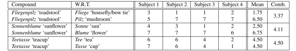
individual compositionality ratings, consists of participants rating the compositionality of a com-pound with respect to each of the individual con-stituents. These judgements were collected within a traditional controlled, pen-and-paper setting. For each compound-constituent pair, 30 native German speakers rated the compositionality of the com-pound with respect to its constituent on a scale from 1 (opaque/non-compositional) to 7 (transpar-ent/compositional). The subjects were allowed to omit ratings for unfamiliar words, but very few did; of the 14,640 possible ratings judgements, only 111 were left blank. Table 1 gives several examples of such ratings. We can see thatFliegenpilz‘toadstool’ is an example of a very opaque (non-compositional) word with respect toFliege‘housefly/bow tie’; it has little to do with either houseflies or bow ties. On the other handTeetasse‘teacup’ is highly composi-tional: it is aTasse‘cup’ intended forTee‘tea’.

Compound W.R.T. Subject 1 Subject 2 Subject 3 Subject 4 Mean Comb.

Fliegenpilz‘toadstool’ Fliege‘housefly/bow tie’ 3 1 1 2 1.75

3.37

Fliegenpilz‘toadstool’ Pilz‘mushroom’ 5 7 7 7 6.50

Sonnenblume‘sunflower’ Sonne‘sun’ 4 3 1 2 2.50

4.11

Sonnenblume‘sunflower’ Blume‘flower’ 7 7 7 6 6.75

Teetasse‘teacup’ Tee‘tea’ 6 6 4 2 4.50

4.50

Teetasse‘teacup’ Tasse‘cup’ 7 6 4 1 4.50

Table 1: Sample compositionality ratings for three compounds with respect to their constituents. We list the mean rat-ing for only these 4 subjects to facilitate examples. The Combined column is the geometric mean of both constituents.

Compound Subject 1 Subject 2 Subject 3 Subject 4 Mean

Fliegenpilz‘toadstool’ - 2 1 2 2.67

Sonnenblume‘sunflower’ 3 3 1 2 2.75

Teetasse‘teacup’ 7 7 7 6 6.75

Table 2: Example whole compositionality ratings for three compounds. Note that Subject 1 chose not to rate Fliegen-pilz, so the mean is computed using only the three available judgements.

3 Methodology

In order to check on the reliability of composition-ality judgements in general terms as well as with re-gard to our two specific collections, we applied two standard cleansing approaches3to our rating data: Z-score filteringis a method for filtering Type I noise, such as random guesses made by individuals when a word is unfamiliar. Minimum Subject Agreementis a method for filtering out Type II noise, such as sub-jects who seem to misunderstand the rating task or rarely agree with the rest of the population. We then evaluated the original vs. cleaned data by one intrin-sic and one extrinintrin-sic task. Section 3.1 presents the two evaluations and the unadulterated, baseline mea-sures for our experiments. Sections 3.2.1 and 3.2.2 describe the cleansing experiments and results.

3.1 Evaluations and Baselines

For evaluating the cleansing methods, we propose two metrics, an intrinsic and an extrinsic measure.

3.1.1 Intrinsic Evaluation:

Consistency between Rating Data Sets

The intrinsic evaluation measures the consistency between our two ratings setsindividual andwhole. Assuming that the compositionality ratings for a compound depend heavily on both constituents, we expect a strong correlation between the two data sets. For a compound to be rated transparent as a

3

See Ben-Gal (2005) or Maletic and Marcus (2010) for overviews of standard cleansing approaches.

whole, it should be transparent with respect to both of its constituents. Compounds which are highly transparent with respect to only one of their con-stituents should be penalized appropriately.

In order to compute a correlation between the whole ratings (which consist of one average rating per compound) and the individual ratings (which consist of two average ratings per compound, one for each constituent), we need to combine the individual ratings to arrive at a single value. We use the geo-metric mean to combine the ratings, which is effec-tively identical to the multiplicative methods in Wid-dows (2008), Mitchell and Lapata (2010) and Reddy et al. (2011b).4 For example, using our means listed in Table 1, we may compute the combined rating for

Sonnenblumeas√6.75∗2.50 ≈4.11. These com-bined ratings are computed for all compounds, as listed in the “Comb.” column of Table 1. We then compute our consistency measure as the Spearman’s

ρrank correlation between these combined individ-ual ratings with the whole ratings (“Mean” in Table 2). The original, unadulterated data sets have a con-sistency measure of 0.786, indicating that, despite the very different collection methodologies, the two ratings sets largely agree.

3.1.2 Extrinsic Evaluation:

Correlation with Association Norms

The extrinsic evaluation compares the consistency

4

Word Example Associations

Fliegenpilz‘toadstool’ giftig‘poisonous’,rot‘red’,Wald‘forest’

Fliege‘housefly/bow tie’ nervig‘annoying’,summen‘to buzz’,Insekt‘insect’ Pilz‘mushroom’ Wald‘forest’,giftig‘poisonous’,sammeln‘to gather’ Sonnenblume‘sunflower’ gelb‘yellow’,Sommer‘summer’,Kerne‘seeds’ Sonne‘sun’ Sommer‘summer’,warm‘warm’,hell‘bright’ Blume‘flower’ Wiese‘meadow’,Duft‘smell’,Rose‘rose’

Table 3: Example association norms for two German compounds and their constituents.

between our two rating sets individual and whole

with evidence from a large collection of associa-tion norms. Associaassocia-tion norms have a long tradiassocia-tion in psycholinguistic research to investigate semantic memory, making use of the implicit notion that asso-ciates reflect meaning components of words (Deese, 1965; Miller, 1969; Clark, 1971; Nelson et al., 1998; Nelson et al., 2000; McNamara, 2005; de Deyne and Storms, 2008). They are collected by presenting a

stimulus word to a subject and collecting the first words that come to mind.

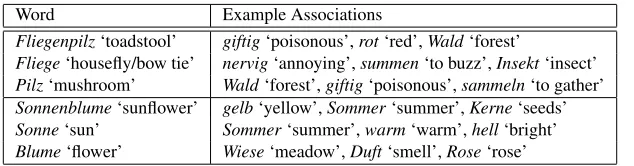
We rely on association norms that were collected for our compounds and constituents via both a large scale web experiment and Amazon Mechanical Turk (Schulte im Walde et al., 2012) (unpublished). The resulting combined data set contains 85,049/34,560 stimulus-association tokens/types for the compound and constituent stimuli. Table 3 gives examples of associations from the data set for some stimuli.

The guiding intuition behind comparing our rat-ing data sets with association norms is that a com-pound which is compositional with respect to a stituent should have similar associations as its con-stituent (Schulte im Walde et al., 2012).

To measure the correlation of the rating data with the association norms, we first compute the Jac-card similaritythat measures the overlap in two sets, ranging from 0 (perfectly dissimilar) to 1 (perfectly similar). The Jaccard is defined for two sets,Aand

B, as

J(A, B) = |A∩B| |A∪B|.

For example, we can use Table 3 to compute the Jaccard similarity betweenSonnenblumeandSonne:

|{Sommer}|

|{gelb,Sommer,Kerne,warm,hell}| = 0.20.

After computing the Jaccard similarity between

all compounds and constituents across the associ-ation norms, we correlate this associassoci-ation overlap with the average individual ratings (i.e., column “Mean” in Table 1) using Spearman’sρ. This cor-relation “Assoc Norm (Indiv)” reachesρ = 0.638 for our original data. We also compute a combined Jaccard similarity using the geometric mean, e.g.

p

J(F liegenpilz, F liege)∗J(F liegenpilz, P ilz),

and calculate Spearman’sρwith the whole ratings (i.e., column “Mean” in Table 2). This correlation “Assoc Norm (Whole)” reachesρ = 0.469for our original data.

3.2 Data Cleansing

We applied the two standard cleansing approaches,

Z-score FilteringandMinimum Subject Agreement, to our rating data, and evaluated the results.

3.2.1 Z-score Filtering

Z-score filtering is a method to filter out Type I noise, such as random guesses made by individu-als when a word is unfamiliar. It makes the sim-ple assumption that each item’s ratings should be roughly normally distributed around the “true” rat-ing of the item, and throws out all outliers which are more thanz∗standard deviations from the item’s mean. With regard to our compositionality ratings, for each itemi(i.e., a compound in thewholedata, or a compound–constituent pair in the individual

data) we compute the meanx¯i and standard devia-tion σi of the ratings for the given item. We then remove all values fromxiwhere

|xi−x¯i|> σiz∗,

● ● ● ● ● ● ● ● ● ● ● ● ● ● ● ● ● ● ● ● ● ● ● ● ● ● ● ● ● ● ● ● ● ● ● ● ● ● ● ● ● ● 0.72 0.73 0.74 0.75 0.76 0.77 0.78 0.79 0.80

N/A 4.0 3.0 2.0 1.0

Maximum Z−score of Judgements

Consistency betw

een r

atings

(Spear

man's rho)

● _{Cleaned Indiv} ● _{Cleaned Whole} ● _{Cleaned Indiv & Whole} (a) Intrinsic Evaluation of Z−score Filtering

● ● ● ● ● ● ● ● ● ● ● ● ● ● ● ● ● ● ● ● ● ● ● ● ● ● ● ● 0.40 0.45 0.50 0.55 0.60 0.65

N/A 4.0 3.0 2.0 1.0

Maximum Z−score of Judgements

Correlation with Association Nor

m Ov

er

lap

(Spear

man's rho)

● _{Assoc Norms (Indiv)} ● _{Assoc Norms (Whole)}

(b) Extrinsic Evaluation of Z−score Filtering

Figure 1: Intrinsic and Extrinsic evaluation of Z-score fil-tering. We see that Z-score filtering makes a minimal dif-ference when filtering is strict, and is slightly detrimental with more aggressive filtering.

σi = 2. If we use az∗of 1, then we would filter rat-ings outside of the range[2−1∗2,2 + 1∗2]. Thus, the resulting newxi would be(1,2,1,1,1)and the new meanx¯iwould be1.2.

Filtering Outliers Figure 1a shows the results for the intrinsic evaluation of Z-score filtering. The solid black line represents the consistency of the fil-tered individual ratings with the unadulterated whole ratings. The dotted orange line shows the consis-tency of the filtered whole ratings with the unadul-terated individual ratings, and the dashed purple line shows the consistency between the data sets when both are filtered. In comparison, the consistency be-tween the unadulterated data sets is provided by the horizontal gray line. We see that Z-score filtering overall has a minimal effect on the consistency of

● ● ● ● ● ● ● ● ● ● ● ● ● ● ● ● ● ● ● ● ● ● ● ● ● ● ● ● ● ● ● ● ● ● ● ● ● ● ● ● ● ● 0.0 0.1 0.2 0.3 0.4 0.5 0.6 0.7 0.8 0.9 1.0

N/A 4.0 3.0 2.0 1.0

Maximum Z−score of Judgements

Fr

action Data Retained

● _Indiv ● _Whole ● _Both Data Retention with Z−score Filtering

Figure 2: The data retention rate of Z-score filtering. Data retention drops rapidly with aggressive filtering.

the two data sets. It provides very small improve-ments with high Z-scores, but is slightly detrimental at more aggressive levels.

Figure 1b shows the effects of Z-score filtering with our extrinsic evaluation of correlation with as-sociation norms. At all levels of filtering, we see that correlation with association norms remains mostly independent of the level of filtering.

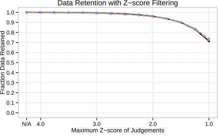
An important factor to consider when evaluating these results is the amount of data dropped at each of the filtering levels. Figure 2 shows the data re-tention rate for the different data sets and levels. As expected, more aggressive filtering results in a sub-stantially lower data retention rate. Comparing this curve to the consistency ratings gives a clear picture: the decrease in consistency is probably mostly due to the decrease in available data but not due to filtering outliers. As such, we believe that Z-score filtering does not substantially improve data quality, but may be safely applied with a conservative maximum al-lowed Z-score.

●

● ●● ●● ●● ●● ●● ●● ●● ●● ●_● ●● ●● ●

●

●

●

0.65 0.70 0.75 0.80

N/A 4.0 3.0 2.0 1.0

Maximum Z−score of Judgements

Consistency betw

een r

atings

(Spear

man's rho)

● _{Cleaned Indiv} ● _{Noisy Indiv}

(a) Removing Indiv Judgements with Uniform Noise

●

● ●● ●● ●● ●● ●● ●● ●● ●●

●

●

●

● ●● ●●

●

●

0.65 0.70 0.75 0.80

N/A 4.0 3.0 2.0 1.0

Maximum Z−score of Judgements

Consistency betw

een r

atings

(Spear

man's rho)

● _{Cleaned Whole} ● _{Noisy Whole}

(b) Removing Whole Judgements with Uniform Noise

Figure 3: Ability of Z-score filtering at removing artificial noise added in the (a) individual and (b) whole judgements. The orange lines represent the consistency of the data with the noise, but no filtering, while the black lines indicate the consistency after Z-score filtering. Z-score filtering appears to be unable to find uniform random noise in either situation.

● ● ● ● _● ● ● ●

●

● ●

● ● ● ● ● ● ● ●

●

● ●

● ● ● ● _● ● ● ● _● ●

●

0.72 0.73 0.74 0.75 0.76 0.77 0.78 0.79 0.80

0.1 0.2 0.3 0.4 0.5 0.6

Minimum Subject−Average Correlation (Spearman's rho)

Consistency betw

een r

atings

(Spear

man's rho)

● _{Cleaned Indiv} ● _{Cleaned Whole} ● _{Cleaned Indiv & Whole} (a) Intrinsic Evaluation of MSA Filtering

● ● ● ● ● ● ● ● ●

●

●

● ● ● ● ● ● ● ● ● ● ●

0.40 0.45 0.50 0.55 0.60 0.65

0.1 0.2 0.3 0.4 0.5 0.6

Minimum Subject−Average Correlation (Spearman's rho)

Correlation with Association Nor

m Ov

er

lap

(Spear

man's rho)

● _{Assoc Norms (Indiv)} ● _{Assoc Norms (Whole)}

(b) Extrinsic Evaluation of MSA Filtering

replaced with a uniform random integer between 1 and 7. That is, roughly 1 in 4 of the entries in the original matrix were replaced with random, uniform noise. We then apply Z-score filtering on each of these noisy matrices and report their average con-sistency with its companion, unadulterated matrix. That is, we add noise to the individual ratings ma-trix, and then compare its consistency with the orig-inal whole ratings matrix, and vice versa. Thus if we are able to detect and remove the artificial noise, we should see higher consistencies in the filtered matrix over the noisy matrix.

Figure 3 shows the results of adding noise to the original data sets. The lines indicate the averages over all 100 matrix variations, while the shaded ar-eas represent the 95% confidence intervals. Surpris-ingly, even though 1/4 entries in the matrix were re-placed with random values, the decrease in consis-tency is relatively low in both settings. This likely indicates our data already has high variance. Fur-thermore, in both settings, we do not see any in-crease in consistency from Z-score filtering. We must conclude that Z-score appears ineffective at re-moving Type I noise in compositionality ratings.

We also tried introducing artificial noise in a sec-ond way, where judgements were not replaced with a uniformly random value, but a fixed offset of either +3 or -3, e.g., 4’s became either 1’s or 7’s. Again, the values were changed with probability of 0.25. The results were remarkably similar, so we do not include them here.

3.2.2 Minimum Subject Agreement

Minimum Subject Agreement is a method for fil-tering out subjects who seem to misunderstand the rating task or rarely agree with the rest of the pop-ulation. For each subject in our data, we compute the average ratings for each itemexcluding the sub-ject. The subject’s rank agreementwith the exclu-sive averages is computed using Spearman’sρ. We can then remove subjects whose rank agreement is below a threshold, or remove thensubjects with the lowest rank agreement.

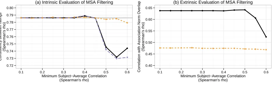
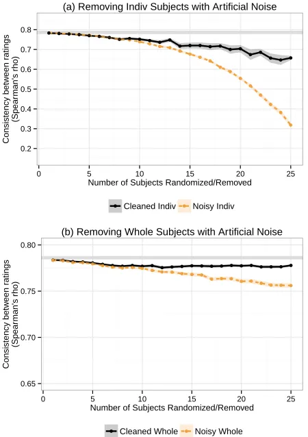
Filtering Unreliable Subjects Figure 4 shows the effect of subject filtering on our intrinsic and extrin-sic evaluations. We can see that mandating mini-mum subject agreement has a strong, negative

im-● ● ● ● ● ● ● ● ● ● ● ● ● ● ● ● ● ● ● ● ● ● ● ● ● ● ● ● ● ● ● ● ● ● ● ● ● ● ● ● ● ● ● ● ● ● ● ● ● ● 0.2 0.3 0.4 0.5 0.6 0.7 0.8

0 5 10 15 20 25

Number of Subjects Randomized/Removed

Consistency betw

een r

atings

(Spear

man's rho)

● _{Cleaned Indiv} ● _{Noisy Indiv}

(a) Removing Indiv Subjects with Artificial Noise

● ● ● ● ● ● ● ● ● ● ● ● ● ● ● ● ● ● ● ● ● ● ● ● ● ● ● ● ● ● ● ● ● ● ● ● ● ● ● ● ● ● ● ● ● ● ● ● ● ● 0.65 0.70 0.75 0.80

0 5 10 15 20 25

Number of Subjects Randomized/Removed

Consistency betw

een r

atings

(Spear

man's rho)

● _{Cleaned Whole} ● _{Noisy Whole}

(b) Removing Whole Subjects with Artificial Noise

Figure 5: Ability of subject filtering at detecting highly deviant subjects. We see that artificial noise strongly hurts the quality of the individual judgements, while hav-ing a much weaker effect on the whole judgements. The process is effective at identifying deviants in both set-tings.

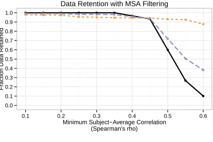
pact on the individual ratings after a certain thresh-old is reached, but virtually no effect on the whole ratings. When we consider the corresponding data retention curve in Figure 6, the result is not surpris-ing: the dip in performance for the individual ratings comes with a data retention rate of roughly 25%. In this way, it’s actually surprising that it does so well: with only 25% of the original data, consistency is only 5 points lower. The effects are more dramatic in the extrinsic evaluation.

● ● ● ● ● ● ●

●

●

●

●

● ● ● _{● ●}

● ● ● ● ●

●

● ● ● ● ● ● _●

●

●

●

●

0.0 0.1 0.2 0.3 0.4 0.5 0.6 0.7 0.8 0.9 1.0

0.1 0.2 0.3 0.4 0.5 0.6

Minimum Subject−Average Correlation (Spearman's rho)

Fr

action Data Retained

● _Indiv ● _Whole ● _Both Data Retention with MSA Filtering

Figure 6: Data retention rates for various levels of mini-mum subject agreement. The whole ratings remain rela-tively untouched by mandating high levels of agreement, but individual ratings are aggressively filtered after a sin-gle breaking point.

the subjects who rated the fewest items since their agreement is more sensitive to small changes. As such, the subjects removed tend to be the subjects with the least influence on the data set.

Removing Artificial Subject-level Noise To test the hypothesis that minimum subject agreement fil-tering is effective at removing Type II noise, we in-troduce artificial noise at the subject level. For these experiments, we create 100 variations of our ma-trices wheren subjects have all of their ratings re-placed with random, uniform ratings. We then apply subject-level filtering where we remove the n sub-jects who agree least with the overall averages.

Figure 5a shows the ability of detecting Type II noise in the individual ratings. The results are un-surprising, but encouraging. We see that increasing the number of randomized subjects rapidly lowers the consistency with the whole ratings. However, the cleaned whole ratings matrix maintains a fairly high consistency, indicating that we are doing a nearly perfect job at identifying the noisy individuals.

Figure 5b shows the ability of detecting Type II noise in the whole ratings. Again, we see that the cleaned noisy ratings have a higher consistency than the noisy ratings, indicating the efficacy of subject agreement filtering at detecting unreliable subjects. The effect is less pronounced in the whole ratings than the individual ratings due to the lower propor-tion of subjects being randomized.

Identification of Spammers Removing subjects with the least agreement lends itself to another sort of evaluation: predicting subjects rejected during data collection. As discussed in Section 2, subjects who failed to identify the fake words or had an over-all low reputability were filtered from the data before any analysis. To test the quality of minimum sub-ject agreement, we reconstructed the data set where these previously rejected users were included, rather than removed. Subjects who rated fewer than 10 items were still excluded.

The resulting data set had a total of 242 users: 150 (62.0%) which were included in the original data, and 92 (38.0%) which were originally rejected. Af-ter constructing the modified data set, we sorted the subjects by their agreement. Of the 92 subjects with the lowest agreement, 75 of them were rejected in the original data set (81.5%). Of the 150 subjects with the highest agreement, only 17 of them were rejected from the original data set (11.3%). The typ-ical precision-recall tradeoff obviously applies.

Curiously, we note that the minimum subject agreement at this 92nd subject was 0.457. Compar-ing with the curves for theindividual ratingsin Fig-ures 4a and 6, we see this is the point where intrinsic consistency and data retention both begin dropping rapidly. While this may be a happy coincidence, it does seem to suggest that the ideal minimum sub-ject agreement is roughly where the data retention rate starts rapidly turning.

Regardless, we can definitely say that minimum subject agreement is a highly effective way of root-ing out spammers and unreliable participants.

4 Conclusion

provides strong evidence that human judgements of compositionality, or at least these particular data sets, are reasonable as gold standards for other com-putational linguistic tasks.

We also find that such ratings can be highly ro-bust against large amounts of data loss, as in the case of aggressive Z-score and minimum subject agreement filtering: despite data retention rates of 10-70%, consistency between our data sets never dropped more than 6 points. In addition, we find that the correlation between compositionality ratings and association norms is substantial, but generally much lower and less sensitive than internal consistency.

We generally find Type I noise to be very diffi-cult to detect, and Z-score filtering is mostly inef-fective at eliminating unreliable item ratings. This is confirmed by both our natural and artificial exper-iments. At the same time, Z-score filtering seems fairly harmless at conservative levels, and probably can be safely applied in moderation with discretion.

On the other hand, we have confirmed that mini-mum subject agreement is highly effective at filter-ing out incompetent and unreliable subjects, as evi-denced by both our artificial and spammer detection experiments. We conclude that, as we have defined it, Type II noise is easily detected, and removing this noise produces much higher quality data. We recom-mend using subject agreement as a first-pass identi-fier of likely unreliable subjects in need of manual review.

We would also like to explore other types of compounds, such as adjective-noun compounds (e.g.

Großeltern ‘grandparents’), and compounds with more than two constituents (e.g. Bleistiftspitzma-chine‘automatic pencil sharpener’).

Acknowledgments

We thank the SemRel group, Alexander Fraser, and the reviewers for helpful comments and feedback. The authors acknowledge the Texas Advanced Com-puting Center (TACC) for providing grid resources that have contributed to these results.5

5_{http://www.tacc.utexas.edu}

References

Collin Bannard. 2005. Learning about the Meaning of

Verb–Particle Constructions from Corpora.Computer

Speech and Language, 19:467–478.

Marco Baroni and Roberto Zamparelli. 2010. Nouns

are vectors, adjectives are matrices: Representing

adjective-noun constructions in semantic space. In

Proceedings of the 2010 Conference on Empiri-cal Methods in Natural Language Processing, pages 1183–1193, Cambridge, MA, October.

Irad Ben-Gal. 2005. Outlier detection. In O. Maimon

and L. Rockach, editors,Data Mining and Knowledge

Discobery Handbook: A Complete Guide for Practi-tioners and Researchers. Kluwer Academic Publish-ers.

Gemma Boleda, Marco Baroni, Nghia The Pham, and Louise McNally. 2013. On adjective-noun compo-sition in distributional semantics. In Proceedings of the 10th International Conference on Computational Semantics, Potsdam, Germany.

Chris Callison-Burch and Mark Dredze, editors. 2010.

Proceedings of the NAACL/HLT Workshop on Creat-ing Speech and Language Data with Amazon’s Me-chanical Turk, Los Angeles, California.

Herbert H. Clark. 1971. Word Associations and Lin-guistic Theory. In John Lyons, editor,New Horizon in Linguistics, chapter 15, pages 271–286. Penguin. Bob Coecke, Mehrnoosh Sadrzadeh, and Stephen Clark.

2011. Mathematical foundations for a compositional distributional model of meaning. Linguistic Analysis, 36(1-4):345–384.

Paul Cook and Suzanne Stevenson. 2006. Classifying Particle Semantics in English Verb-Particle

Construc-tions. InProceedings of the ACL/COLING Workshop

on Multiword Expressions: Identifying and Exploiting Underlying Properties, Sydney, Australia.

Simon de Deyne and Gert Storms. 2008. Word associ-ations: Norms for 1,424 dutch words in a continuous task.Behavior Research Methods, 40(1):198–205.

James Deese. 1965. The Structure of Associations in

Language and Thought. The John Hopkins Press, Bal-timore, MD.

Wolfgang Fleischer and Irmhild Barz. 2012.

Wortbil-dung der deutschen Gegenwartssprache. de Gruyter. Edward Grefenstette, G. Dinu, Y. Zhang, Meernoosh

Sadrzadeh, and Marco Baroni. 2013. Multi-step re-gression learning for compositional distributional

se-mantics. In Proceedings of the 10th International

Conference on Computational Semantics, Potsdam, Germany.

Jonathan I. Maletic and Adrian Marcus. 2010. Data

cleansing: A prelude to knowledge discovery. In

O. Maimon and L. Rokach, editors, Data Mining

and Knowledge Discovery Handbook. Springer Sci-ence and Business Media, 2 edition.

Diana McCarthy, Bill Keller, and John Carroll. 2003. Detecting a Continuum of Compositionality in Phrasal

Verbs. InProceedings of the ACL-SIGLEX Workshop

on Multiword Expressions: Analysis, Acquisition and Treatment, Sapporo, Japan.

Timothy P. McNamara. 2005. Semantic Priming:

Per-spectives from Memory and Word Recognition. Psy-chology Press, New York.

George Miller. 1969. The Organization of Lexical Mem-ory: Are Word Associations sufficient? In George A.

Talland and Nancy C. Waugh, editors, The

Pathol-ogy of Memory, pages 223–237. Academic Press, New York.

Jeff Mitchell and Mirella Lapata. 2010. Composition in Distributional Models of Semantics. Cognitive Sci-ence, 34:1388–1429.

Douglas L. Nelson, Cathy L. McEvoy, and Thomas A.

Schreiber. 1998. The University of South Florida

Word Association, Rhyme, and Word Fragment Norms.

Douglas L. Nelson, Cathy L. McEvoy, and Simon Den-nis. 2000. What is Free Association and What does it

Measure? Memory and Cognition, 28:887–899.

Siva Reddy, Ioannis P. Klapaftis, Diana McCarthy, and Suresh Manandhar. 2011a. Dynamic and Static

Pro-totype Vectors for Semantic Composition. In

Pro-ceedings of the 5th International Joint Conference on Natural Language Processing, pages 705–713, Chiang Mai, Thailand.

Siva Reddy, Diana McCarthy, and Suresh Manandhar. 2011b. An Empirical Study on Compositionality in

Compound Nouns. InProceedings of the 5th

Interna-tional Joint Conference on Natural Language Process-ing, pages 210–218, Chiang Mai, Thailand.

Sabine Schulte im Walde, Susanne Borgwaldt, and Ronny Jauch. 2012. Association Norms of German

Noun Compounds. InProceedings of the 8th

Interna-tional Conference on Language Resources and Evalu-ation, pages 632–639, Istanbul, Turkey.

Richard Socher, Eric H. Huang, Jeffrey Pennington, An-drew Y. Ng, and Christopher D. Manning. 2011. Dy-namic Pooling and Unfolding Recursive Autoencoders for Paraphrase Detection. In Advances in Neural In-formation Processing Systems 24.

Claudia von der Heide and Susanne Borgwaldt. 2009. Assoziationen zu Unter-, Basis- und Oberbegriffen.

Eine explorative Studie. In Proceedings of the 9th

Norddeutsches Linguistisches Kolloquium, pages 51– 74.