Munich Personal RePEc Archive
Exact Methods for Path-Dependent
Credit Exposure
Zhou, Richard
Wells fargo
25 May 2015
Online at
https://mpra.ub.uni-muenchen.de/64647/
1
Exact Methods for Path-Dependent Credit Exposure
Richard Zhou
1Wells Fargo
May 25, 2015
Summary
Path dependent counterparty credit risk exposure modeling poses challenges. In this paper, we present models for consistent and accurate estimation of counterparty credit exposure involving barrier option and European swaption under the general Monte Carlo simulation framework. In particular, we discuss how to consistently estimate the pathwise swaption exercise probability and accurate monitoring of barrier crossing. We present exact formulation for standalone expected exposure and potential future exposure for swap, swaption and barrier option without monte carlo simulation. The exact formulation is of practical importance to computing standalone exposure profiles, exposure model validation and system benchmarking.
1 Introduction
Modeling counterparty credit risk exposure for path-dependent derivatives poses significant challenges. A major issue is that the actual type of a path-dependent instrument at future times is unknown at the valuation date. This is referred to as instrument aging which differs from the shortening of the instrument’s time-to-maturity because time-to-maturity change does not alter instrument type.
Broadly speaking, there are two kinds of path-dependency. One can be termed as automatic exercise, or European style exercise, where the instrument either terminates or becomes an instrument of a different type if some predefined condition is met at a specific time or during the life of the option. Under automatic exercise, no decision is required and exercise is automatic. Examples of automatic exercise include barrier options and physically settled European swaptions. The other can be loosely called optimal exercise, or American style exercise, where the exercise decision is based on the principle of payoff maximization. Examples include American and Bermudan style options. Modeling optimal exercise is much more involved than modeling automatic exercise. In this paper, we focus on the automatic exercise.
Barrier options and European swaptions are good examples of path-dependent instruments of the automatic exercise. A barrier option is knocked out or in if the underlying reaches the barrier level during the life of the option. Once the barrier is hit, the option type changes, and so does the exposure. The exposure critically depends on the timing of barrier hitting which is unknown at the exposure valuation time. European swaption depends on the value of the underlying swap at the expiry date. In this case, the timing is known, but the swap value is unknown at the exposure valuation time. Therefore, a key issue to accurate computation of barrier option exposure is accurate determination of the barrier hitting time, whereas for European swaption, it is the accurate and consistent determination of the swaption exercise probability. Here, consistency means that the exercise probability must be consistent with the swap pricing. This paper aims to address these two issues.
1
Email: rzhou50@gmail.com. The opinions in this paper are the author’s own and are not in any way
2
Lomibao and Zhu (2006) proposed a conditional valuation method for the type of path-dependent options whose future values can be expressed as either a sum or a product of two terms where one term depends only on the path history and the other term is the future mark-to-market value of the option and is independent of the history. They described the model based on the Direct-Jump-to- Simulation (DJS) scenario generation approach.
With DJS, the scenario at time t is generated independently whereas with the pathwise approach an entire path is simulated. While the two approaches theoretically generate the same distribution, we demonstrate that DJS barrier survival probability does not decrease with time.
A potential issue with using a single lognormal swap rate model for swaption exposure in the conditional approach is that a single swap rate model may be inconsistent with the swap pricing for the entire swap life, as the number of payments on the swap decreases as passage of time.
This paper is written with three goals in mind. First, it presents a model for the pathwise probability at which a European swaption would be exercised into the underlying swap. Our model is based on a short rate model so that the pathwise the pathwise exercise probability is consistent with the pathwise swap value. Second, it discusses a pathwise approach for the barrier hitting probability. This approach takes into account the information of the full monte carlo path. It demonstrates that the pathwise hitting probability can be much different than that of DJS. We demonstrate that the DJS approach is not theoretical sound as the barrier survival probability does not monitonically decrease with time. Third, it describes exact methods for the calculation of standalone exposure profiles under a simple model framework, without monte carlo. In practice, the exact exposure profiles can be used to estimate standalone exposure, and to benchmark CCR system in both development and validation as monte carlo results must converge to the exact results.
The rest of the paper is organized as follows. Section 2 outlines exposure definitions and formulations. We describe the formula for the generalized Brownian motion (BB) based on a mean-reverting process. To the author’s knowledge, this result has not appeared in literature. Section 3 describes exact methods for standalone expected exposure (EE) and future potential exposure (PFE) for forward and tail interest rate swap. For the tail swap, the accrued interest is treated as stochastic. Section 4 describes a method for estimating the European swaption exercise probability consistent with the underlying swap valuation, and exact swaption EE and PFE profiles. In section 5, we discuss an accurate method for barrier option exposure calculation. Section 6 concludes the paper. Details of derivation are provided in the appendixes.
2 Exposure Definition
We shall use superscripts P and Q to denote the scenario and the pricing measures, respectively. Since pricing is usually under the risk-neutral (RN) measure, Q generally refers to the RN measure. The scenario measure P may be either real-world (RW) or RN depending on the
context. For instance, trading book CVA requires RN so P is RN, whereas PFE and EE for capital purpose generally require RW scenarios so P should be RW.2
Consider a counterparty portfolio with cashflow on dates . The portfolio mark-to-market value at future time t is
(2.1)
2
3
where is the next cashflow date from t. Note that , reflecting the assumption that cashflow at default time should be part of the exposure. is the augmented P-measure filtration generated by scenario path. This means that contains the information up to t along a specific path. Alternatively, we can think of as path identification.
is the stochastic discount factor under the Q-measure which differs from
the zero-coupon bond (ZCB) price defined as
. (2.2)
In the scenario/revaluation model framework, an important issue is the consistency between scenario and pricing. As the pricing is conditioned on the scenario path , should be consistent with the scenario interest rate curves as clearly indicated in (2.1) and (2.2).
When using a term structure model (eg, LMM and HJM model) to generate interest rate scenario, by construction, the scenario filtration contains the whole simulated yield curve which can be used as the initial yield curve for arbitrage pricing model. As a result, matches exactly the scenario interest rate curve when conditioned on , provided that the pricing model is an exogenous model. Take, for example, the Hull-White model (Hull and White 1990) as the pricing model. The mean-reversion speed and the volatility are calibrated at time 0.3 The reversion level can then be used to match the scenario yield curve at time t.
If the interest rate scenarios are generated by a short rate model, then the short rate , not the yield curve,is the risk scenario. The short rate says nothing about the scenario yield curve at time t. In this case, one strategy is to calibrate the pricing model to the initial market condition, which is then used to generate the yield curve defined in (2.2). This is the strategy we assume to derive the exact exposure formulas in this paper.
The current exposure at time t is defined as . The expected exposure (EE) and negative expected exposure (NEE) are defined by
(2.3)
EE is the expected credit loss with no recovery should the counterparty default, and NEE is the expected benefit to the bank should the bank default. NEE is used for DVA calculation. It is important to note that, as indicated by (2.1) and (2.3), the portfolio value is evaluated under the measure Q while EE and NEE are evaluated under the measure P.
The portfolio value is conditioned on augmented scenario filtration , and hence depends on a specific scenario path, ie, is pathwise. is the average value of over all such scenario paths conditional on the information at time 0. As such, is a deterministic function of time.
The PFE for confidence level α is defined as
(2.4)
3
The mean-reversion speed is difficult to calibrate because it is sensitive to the input data and its impact on the short end of the yield curve is weak. The latter is due to the fact that in a diffusion model, the near term is dominated by diffusion. Therefore, the mean-reversion has virtually no effect on the short-term
4
When the portfolio value has a continuous distribution, PFE can be computed by solving
(2.5)
(2.4) shows that is the zero-floored -percentile of the portfolio value distribution at t
seen at time 0. The second expression in (2.4) shows that PFE is similar to VaR as both are quantile measures. In practice, (2.5) is more convenient to use.
Remark 2.1:Contrary to some belief, can actually be less than , because dose not account for the distribution tail beyond the confidence level
, whereas
accounts for the entire distribution. Consider a stock forward contract, the EE and PFE are, respectivelyand
where
and
. If and , we have , which means for all .Remark 2.2: (2.8) is convenient for analytical expression of option exposure as cashflow on an option is positive.
In the above discussion, we did not impose any relationship between the P and Q measures. It is desirable to treat these two measures as distinct because the scenario model may be calibrated to the historical volatility while the pricing model is calibrated to the market implied volatility.
Proposition 1: Let follow the mean-reverting process
(2.9)
Then the distribution of conditional on and , where , is a generalized Brownian bridge (BB) with the distribution
(2.10)
where is the cumulative normal distribution with mean and variance
(2.11)
(2.12)
(2.13)
(2.14)
Proof is given in appendix A. Here, we discuss some properties of the conditional distribution
due to mean reversion.
For the standard Brownian motion , the conditional distribution is also given by (2.10) with the following properties (Glasserman 2004, p. 84 ):
- , where
, is a linear function of .
5
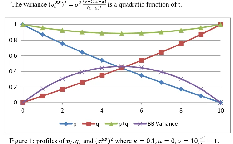
- The varianceis a quadratic function of t.
Figure 1: profiles of and where
.
The mean reversion introduces some complexity. Formulas (2.11)-(2.14) show that
- The mean is not a linear function of time. Nor is it a weighted average of and ,
since , as demonstrated in figure 1.
- The mean function is independent of the initial value , but is dependent on the mean reversion level . The term can be viewed as convexity adjustment.
- The variance is not a quadratic function of t.
- In the limit , the process (2.8) approaches the standard Brownian motion, as
; and
.
- At the endpoints of the Brownian bridge , , thus we have
, and . This means at .
Since , (2.10) derived from the mean-reversion process is not a Brownian bridge in the traditional sense. The extra term can be interpreted as a convexity adjustment. For positive mean reversion level , this convexity is positive. The maximum value is at the midpoint
.
3 Interest Rate Swap Exposure
Fixed-for-floating interest rate swaps and European swaptions are amongest most widely traded OTC fixed income derivatives. Global banks have substantial swap books. Swaps are also convenient cases for counterparty exposure model validation due to its simplicity. While
frequently used as an example in literature and often among the first instruments to be covered in a newly developed CCR system, there still appears to be a practical need for a detailed, rigorous exposition on the profile of swap value and exposure.
In this section, we discuss in detail swap valuation and exposure. We pay special attention to the jump in swap value across a payment date because it is why swap exposure profile exhibit a sawtooth pattern.
0 0.2 0.4 0.6 0.8 1
0 2 4 6 8 10
[image:6.612.111.483.74.305.2]6
Consider an interest rate swap exchanging the Libor for a fixed rate K. The swap starts at and ends at , with the floating rate payment dates and the fixed rate payment dates . Assuming Libor fixing and discounting, the future mark-to-market swap value to the fixed rate payer is
(3.1)
where . In (3.1), and ,0 are indexes of the next fixed and floating rate payment dates, respectively. and are continuous from the left in order for the accrued interests to be included in the exposure. If we assumes that the coupon is paid immediately before default and hence is not included in the exposure, then . With this definition,
and would be right-continuous with left-limit. Since , the forward swap valuation and tail swap valuation in (3.1) are consistent.
Since t is a simulation date, the zero-coupon bond is known for all T. But is unknown if , the last floating rate payment date prior to t, is not a simulation date. As a result, needs to be either approximated or modeled. Stein and Lee (2010) assumed
, the forward zero-coupon bond value seen at time 0, which is
equivalent to assuming , the time 0 forward rate. Later in this paper, we will discuss consistent valuation of .
In (3.1), and are values of a forward swap and a tail swap, respectively. The tail swap can be expressed as a forward swap starting at plus a net interest accrued to
. For simplicity, we assume that any fixed date is also a floating,
which implies . Thus
(3.2)
The top line in (3.2) is the value of the spot -maturity swap with the floating payment dates
and the fixed rate payment dates . The bottom line represents
the net accrued interest from the last floating and fixed dates to t which we will discuss below.
Notice that is the spot Libor for the time period and is known when conditioned on , the bottom line in (3.2) can be written as
7
(3.3) shows that the net accrued interest at time t is equal to the floating coupon of the original swap for adjusted for the portion that is included in the new swap minus the fixed coupon accrued from the last fixed payment date . It is easy to see that if , then , the full net coupon on the original swap, whereas if , then . In other words, immediately prior to a coupon payment date, is the full accrued coupon, whereas immediately after a payment, the accrued interest is zero.
Put another way, is continuous everywhere except at the coupon payment dates and . Let T be either a floating payment date or a fixed payment date , then the swap value is left continuous, , and right limited, . This is a consequence of the definitions of and . It is easy to verify that if is a payment date for both fixed and floating legs.
The change in swap value across a floating rate payment date is
(3.4)
(3.4) implies that the pathwise value of a payer swap decreases by after a float payment (one less future receipt), and increases by after a fixed payment (one less future payment). The jump magnitude depends on the difference between the fixed and floating rates and their respective accrued periods. This jump is the reason why swap exposure profile typically exhibits a sawtooth pattern.
The change in the pathwise swap value over the time interval is
(3.5)
where . (3.5) is due entirely to diffusion effect and passage of time. Its effect on the exposure profile is gradual and smooth.
Define the forward swap rate and annuity for a -maturity swap that starts at with fixed payment dates and floating payment dates
, (3.6)
The forward swap rate for the original swap is , and the swap rate for the first line of (3.2) is . With (3.6), we can recast the swap value (3.1) into
8
By virtue of (2.3) and (3.1), the standalone EE for the payer swap is
(3.8)
where
(3.9)
A positive (negative) NAI reduces (increases) and hence increases (decreases) the exposure of the tail swap. It is possible for to be negative when K is low or is high. This indicates that a swap rate model for the tail swap EE must be able to handle the possibility of negative swap rate.
It is important to point out that although in (3.8)resembles a European swaption, but it is not, as it is the undiscounted expectation.
Brace and Womersley (2000) showed that is a low variance martingale and hence can be approximated by the time 0 value . Thus, the effective strike can be approximated as
(3.10)
The second part of (3.8) and (3.10) suggest that could be considered as a forward starting swaption with the strike being a linear function of . This is an interesting research topic on its own that is more challenging than its equity counterpart as it involves both Libor and spot swap rate .
In the remainder of this section and the next section, we discuss an exact model for the exposure profiles for standalone swap and European swaption. We assume that the interest rate scenarios are generated by the Vasicek model (B.1) and the zero-coupon bond price (2.2) is calculated using the one-factor Hull-White model (B.2)-(B.4). in the following, we present the main results and provide the detailed derivation in appendices B and C.
The expected swap exposure is defined by
(3.11)
Under the one-factor model framework, we have
9
(3.13) where and the tail swap EE (3.13) follows (B.14) and (B.23), respectively.
The swap PFE profile is defined as
(3.14)
The forward swap PFE is
(3.15)
The tail swap PFE is where m is obtained by solving the integral equation
(3.16)
Equation (3.16) follows (B.26).
Remark 3.1: The exact formulations (3.11)-(3.16) have several utilities. One is that they can be used in CCR system development by providing benchmark solution. Another usage may be that it can be used to estimate standalone exposure and to perform sensitivity analysis.
Remark 3.2: The swap valuation above assumes the single curve paradigm where the fixing curve is the same as the discount curve. The current standard swap pricing uses the multi-curve paradigm (Bianchetti 2010). The exact method can be extended to OIS framework with minor modification, because the Jamshidian method is still applicable.
4
Physically Settled European Swaption
Exposure
Consider a swap-settled European payer swapion, its value after the swaption expiry date depends on whether the swaption is exercised into the swap, which in turn depends on the swap value at the expiry date being positive. However, future swap value is unknown at time 0. Therefore, a key element of modeling physically settled European swaption exposure is accurate estimation of the swaption exercise probability.
Suppose that the swap trade terms are the same as specified in the previous section, and the strike rate is K. The future value of the European swaption is
10
where is the indicator function. The second formula in (4.1) means that if the swap value at is positive, the swaption is exercised and becomes a tail swap after , where the exposure persists until the swap maturity .
The standard front office model for European swaption is the Black-Scholes model
(4.2)
where the forward swap rate and the annuity function are define in (3.6), and
(4.3)
Clearly, and are evaluated on the same monte carlo path. When is a simulation node, is known so we know whether there is a swap on that path after . However, a practical CCR system has a fixed simulation date grid, while a typical portfolio contains many European swaptions, implying that most swaption maturities are generally not on the simulation date grid, and hence the pathwise swaption exercise indicator must be estimated. Since this indicatoris a pathwise variable, it is computed once per path.
Let the simulation date grid be denoted by and assume , the indicator under the P-measure may be directly sampled conditional on . Given that , this indicator takes value 1 with probability . Thus, (4.1) can be expressed as
(4.4)
Direct simulation is inefficient in large scale computation, a practical approach is to estimate the conditional exercise probability .
In an influential paper, Lomibao & Zhu (2006) proposed a conditional valuation approach for modeling EE of path-dependent instruments. Their method is intended for the type of path dependent option where the future value of the option can be expressed as either a product (cf. (4.4)) or a sum of two terms. One term is the future MTM value and the other term depends only on the path history.4 Here, the future MTM value is the price at a future date of a newly issued option of the same type as the original option, and hence is independent of the path history. The path history dependent term is essential to exposure calculation as it determines the product type. The central theme of the method is to use the Brownian bridge to estimate the path-dependent term. For the swaption exercise probability , the method assumes that all the co-terminal -maturity swap rates follow the same lognormal process. This enables to link the swap rates of two distinct co-terminal swaps via the relation
4
11
. If is known from the simulation,
can be estimated using the Brownian bridge between 0 and the simulation date .
The method is elegant, simple and efficient. However, for physically settled European swaption, it lacks theoretical justification as it may be inconsistent with the swap pricing. First, is the forward swap rate of an N-period swap underlying the swaption, and is the forward swap rate for a period swap. (3.6) indicates that and generally cannot follow the same lognormal process, because of different annuity function. To illustrate the point, consider a 6-month swaption into a one-year swap receiving 6 month Libor flat with semi-annual payment. Suppose the simulation time nodes are 6 months apart so . is the one-year swap rate which is a weighted average of two adjacent forward 6-month Libor spanning the one-year swap, while is the 6-month forward Libor for the last 6-month of the one-year swap. Clearly, the one one-year swap rate and the 6-month Libor generally do not follow the same process. Second, since and represent swaps of different maturities, they should have different volatilities. This raises the question of what volatility to use for the Brownian bridge model. Third, these issues are likely exacerbated by the fact that a typical counterparty portfolio contains many swaptions.
The above discussion suggests that should be consistent with the swap pricing, hence using a swap rate model may not be appropriate. In the following, we propose a simple, practical method for consistent calculation of the European swaption exercise probability.
Proposition 2: Suppose that the scenario interest rate follows the process
(4.5)
The payer European swaption exercise probability conditional on is5
(4.6) where is an increasing function and is the critical rate such that , and
and are given in (2.12)-(2.14).
Proof: The swap value (3.1) at the swaption expiry date is
(4.7)
Based on a method developed by Jamshidian (1989), we can find a unique value such that
iff . In other words, the payer swaption is exercised iff . The
critical rate is unique for a given swap, and needs to be computed only once.
5
12
By virtue of proposition 1, the conditional distribution of is where the mean and the variance are given by (2.10)-(2.13). Since , proposition 1 implies
(4.8)
Q.E.D.
Let , (4.8) implies that if . The same holds for . These limiting cases indicate that (4.8) is consistent with the case where is a simulation date so we know for sure whether the swaption is exercised. Since the probability of one or zero can only be attained at the two end points, the swaption exposure after the expiry date must be strictly smaller than the exposure of the underlying tail swap.
For the non-trivial case where , (4.8) indicates that the higher are the values of
and/or , the greater is the exercise probability, and vice versa. The interest rate volatility is important to the exercise probability as , regardless of the values of and . Therefore, (4.4) indicates that, for large interest rate volatility, we should expect the residual swaption value to be equal roughly half of that of the underlying swap. For small volatility, the exercise probability is close to one if
and close to zero otherwise. Finally, a high mean-reversion
level alsoincreases the exercise probability.
Substituting (4.4) into (2.3), the EE profile of a standalone European swaption is
(4.9)
Under the scenario and pricing models of (B.1) and (B.2), we have (cf. equation (C.16))
(4.10)
For a payer swaption, an increase in the interest rate results in an increase in the swaption value. Therefore, we have
(4.11)
The swaption PFE for follows equation (C.16),
13
5 Barrier Option Exposure
A barrier option, including one-touch option, is path-dependent. If the underlying state variable reaches some pre-defined barrier level during the life of the barrier option, the option either ceases to exist (knocked out) or becomes a standard European option (knocked in). Modeling barrier option exposure is complicated because the future instrument type of a today’s barrier option depends on what happens between now and then. In other words, barrier option exposure depends on the instrument aging. In the previous section, we discussed a model for the swap-settled European swaption exposure. European swaption exposure calculation requires monitoring the underlying swap value only at the option expiry date. In contrast, barrier option exposure requires continuous monitoring of the entire option life.
Consider a European up-and-out stock call option with rebate (UOR) with the terminal payoff
(5.1)
where is the running maximum of the stock price, H is the barrier level, is the strike, and R is the rebate amount if the stock price crosses H before the expiry date T. When , (5.1) represents a European capped option where it is a call option but pays
should the barrier be breached before expiration, capping the maximum payoff at .
The future MTM price of the UOR option is
(5.2)
Equation (5.2) represents the price of a new UOR option issued at time t when stock price is . The first term is a standard up-and-out barrier option that pays nothing if the barrier is crossed during the life of the option. The second term is a one-touch option representing a contingent rebate. It is emphasized here that depends only on the spot price provided . Assuming the stock pays no dividend, in the Black-Scholes world, we have (Shreve 2004, p. 307)
(5.3)
where
with
.
When it comes to modeling barrier option exposure, two issues must be addressed. The first is the determination of the option type at simulation dates. This can partially be resolved by pathwise simulation. If the stock price exceeds the barrier H on any simulation date, the barrier option ceases to exist. However, stock price monitoring at simulation dates dose not account for the possibility that the stock price may cross the barrier between simulation dates, especially when simulation dates are far apart. This leads to the second issue, quantification of the pathwise barrier survival probability, which is the focus of this section. The lack of underlying state variable monitoring is a main reason that pathwise method is preferable to the DJS.
14
(5.4)
The future value of a today’s UOR option is a weighted average of a new UOR option and the rebate depending on whether the stock has hit the barrier by that time. If , the UOR option survives and the value is given by (5.2). Otherwise, the option has been knocked out and the value is the time t value of the rebate R.
Assuming continuous monitoring, the survival indicator takes value 1 with the conditional barrier survival probability . Hence, the future value of the UOR option is given by
(5.5)
where path history determines the conditional survival probability . Given a simulation date grid , the stock price at a simulation date is known from the stock path simulation. For example, we know the stock price on every simulation date of the path . If for some k, then at .
The discrete monitoring of barrier crossing time ignores the possibility that the barrier may be crossed between simulation dates. For barrier option exposure calculation, monitoring stock price at the simulation dates is insufficient.
Assuming that the real-world stock price follows a lognormal process
(5.6)
Conditional on and , is a Brownian bridge for . The survival probability is then the probability of the maximum of the Brownian bridge staying below
H. This conditional probability is (Glasserman 2004)
(5.7)
As expected, the conditional survival probability decreases as the stock volatility increases since a higher volatility makes barrier crossing more likely. In addition, the closer to H is and/or , the smaller is the conditional survival probability as it is more likely that the stock price crosses the barrier. The pathwise barrier survival indicator at can be calculated recursively as
(5.8)
where, by definition, . Since is available from the stock price path simulation, we have if for some .
15
depends only on and has no knowledge of what happened prior to . The DJS conditional survival probability is given by
.
[image:16.612.104.490.74.325.2]
Figure 2: Comparison of pathwise and DJS survival probability where . The stock price crosses the barrier at . Figure 2 shows a comparison of the two approaches for a particular stock price path. It is interesting to see that the difference between the two methods is so significant that cannot be ignored. We summarize the major difference:
- The difference between the approaches is too significant to ignore, even without hitting the barrier.
- The DJS survival probability is not a decreasing function of time, violating the intuition that the chance of surviving cannot increase with passage of time.
- The DJS survival probability is not zero after the barrier has been breached.
As a result, we recommend the pathwise approach in the calculation of barrier option exposure.
Because the UOR option value (5.4) is always positive, the standalone EE is
(5.9) where (5.10)
It is well known that (Musiela & Rutkowski 1997, p. 470)
(5.11) 0 20 40 60 80 100 120 140 0 0.1 0.2 0.3 0.4 0.5 0.6 0.7 0.8 0.9 1
0 0.25 0.5 0.75 1 1.25 1.5 1.75 2
S to ck Pr ic e S u rv iv al Pr o b ab il ity
16
The P-measure joint density function of is (Shreve 2004)
(5.12)
Recognizing that depends only on and , we have an exact EE formula for UOR option,
(5.13)
Carrying out the inner integral analytically, we obtain
(5.14)
(5.14) can be calculated on a finite interval because dominates as .
(5.9), (5.11) and (5.14) form an exact model for standalone EE of UOR option. The only model dependent part is the scenario model (5.6) which is widely used in the financial industry for stock price scenario generation. (5.14) is exact so it can be used to benchmark simulation based EE.
The risk-neutral standalone EE can be simplified to
(5.15)
Formula (5.15) is based on the law of iterated expectation and the following relations,
(5.16)
6 Conclusions
In this paper, we accomplished three goals. First, we presented a model for estimating the European swaption exercise probability in the monte carlo framework that is consistent with the underlying swap. The consistency is referred to as that the swap value used for swaption exercise decision and the underlying swap value come from the same model so that they are consistent pathwise. The method is model specific, but it may be adapted to other model setting.
Second, we discussed a pathwise method for barrier option survival probability. We demonstrated that pathwise method is superior to the DJS method, for an important reason which is that the DJS produces barrier survival probability that does not decrease with time. We also showed that the difference in the survival probability between the pathwise and DJS is too significant to ignore.
17
7 References
1. Bianchetti, M. (2010). Two curves, one price. Risk Magazine. July.
2. Brace, A. and Womersley, R. S. (2000). Exact fit to the swaption volatility matrix using semidefinite programming. Working paper presented at ICBI Global Derivatives Conference, Paris.
3. Brigo, D., Buescu, C. and Morini, M. (2011). Impact of the first to default on bilateral CVA. Working paper.
4. Brigo, D., Morini, M. and Pallavicini, A. (2013). Counterparty Credit Risk, Collateral and Funding. Wiley Finance.
5. Glasserman, P. (2004). Monte Carlo Methods in Financial Engineering. Springer.
6. Hull, J. and White, A. (1990). Pricing interest-rate derivative securities. The Review of Financial Studies, Vol. 3. No. 4. pp. 573-592.
7. Jamshidian, F. (1989). An exact bond pricing formula. Journal of Finance. 44,pp. 205-209. 8. Lomibao, D. and Zhu, D. (2006). A Conditional Valuation Approach for Path-Dependent
Instruments. Wilmott magazine.
9. Musiela, M. and Rutkowski, M. (1997). Martingale Methods in Financial Modeling.
Springer.
10. Shreve, S. E. (2004). Stochastic Calculus for Finance II. Springer.
11. Stein, H. and Lee, K. P. (2010). Counterparty and Credit Risk. Bloomberg.
12. Vasicek, O. (1977). An equilibrium characterization of the term struure. J. Financial Economics. 5, pp. 177-188.
Appendix A: Brownian Bridge for Mean-Reverting Brownian Motion
The solution to the process (2.8) is(A.1)
where is a standard normal random number and
(A.2)
The covariance function is
(A.3)
Let , the random variables and are joint normal with the covariance matrix
The distribution of conditional on and is given by (Glasserman 2004)
(A.4)
where the mean and the variance of the Brownian bridge are
18
(A.6)
(A.7)
After some mathematical manipulation, we obtain
(A.8)
(A.9)
(A.10)
Q.E.D.
Note that the method can be extended to where are deterministic functions of time, e.g., the Hull-White model.
Appendix B: Exact Swap Exposure Profile
Assuming that the interest rate scenarios are generated by the one-factor Vasicek model (Vasicek 1977), and the zero-coupon bond is priced using the one-factor Hull-White model (Hull &White 1990).
Under the one-factor Vasicek model, the scenario short rate is given by
(B.1)
where is the standard normal variate, and is the initial value.
Using the one-factor Hull-White model, the zero-coupon bond price (2.2) is
(B.2)
where
(B.3)
The function can be calibrated to the initial yield curve , in which case,
(B.4)
Using (2.3) and (2.5), the EE and PFE profiles of a swap are, respectively,
(B.5)
(B.6)
19
(B.8)
where for the forward swap and for the tail swap, and
(B.9)
is a function of the scenario short rate as the zero-coupon bond uses (B.2). Notice that PFE is positive so it is floored at zero.
Based on a method by Jamshidian (1989), it can be shown that for forward swap where , there is a unique value which depends only on m, such that
(B.10)
For each simulation time t, is obtained by solving (B.10). The root finding is efficient for
is given by (B.2). (B.10) implies that only the part of the distribution where contributes to the EE. This is expected as the payer swap benefits from an increase in interest rate. Whereas the interest rate effect is reversed for a receiver swap where the EE contribution comes from .
Similarly, for tail swap where and a given , there is a unique value such that
(B.11)
Using (B.2)-(B.4), we solve (B.11) to obtain
(B.12)
In the following, we set when calculating EE defined in (B.5)-(B.6), and when calculating PFE defined in (B.7)-(B.8).
Having solved for , (B.5) becomes
(B.13)
where
(B.14)
for maturity .
20
(B.15)
Due to the presence of stochastic accrued interest, we must consider the correlation between and , when modeling the tail swap exposure.
Using the critical value defined in (B.12), we first rewrite (B.6) into
(B.16)
where are given by (B.9), (B.12) and (B.2).
Notice that the conditional distribution of given is (Glasserman 2004)
(B.17)
where
and (B.18)
(B.19)
with and being defined in (B.1).
Using the conditional distribution (B.17), we have
(B.20)
(B.21)
where
(B.22)
21
(B.23)
where .
For a given , (B.12) implies the set relation
(B.24)
Hence, (B.8) can be written as
(B.25)
where the inner expectation is given by (B.20) with 0 replaced by . We obtain an exact equation for calculating tail swap PFE
(B.26)
where the expectation is with respect to . The tail swap PFE is defined as
(B.27)
Note that the integrals in (B.23) and (B.26) can be carried out on a finite domain to any specified accuracy.
Remark B.1: It is preferable to use an exogenous model to generate the real-world interest rate scenarios, as the scenario distribution should be close to the historical one, and to avoid frequent re-calibration. On the other hand, for CVA calculation, it is natural to use the same interest rate model for both scenario and pricing. Notice that the method here is equally applicable when replacing (B.1) with the one-factor Hull-White model.
Appendix C: Exact Swaption Exposure Profile
The tail portion of the swaption exposure profiles at time can be formulaed as
(C.1)
(C.2)
In our one-factor model framework, (B.10) implies the set relation
22
Based on (B.24) and (C.3), (C.1) and (C.2) become
(C.4)
(C.5)
with .
To lighten the notation, we use subscripts 1,2,3 to represent the time instances . Defining which follows the trivariate normal distribution, and
. With the simplified notation, (C.4) and (C.5) can be rewritten as
(C.6)
(C.7)
It can be shown that
(C.8)
(C.9)
(C.10)
where
(C.11)
(C.12)
(C.13)
(C.14)
Finally, we have for EE
23
PFE is obtained as
where (C.16)
Remark C.1:Compared (B.16) with (C.4) and (B.25) with (C.5), we see that the dimension of the swaption exposures is increased by 1 due to the term as we need to consider three correlated interest rates and , instead of two correlated rates and
for the tail swap exposure as is irrelevant for the tail swap.
Remark C.2: The above results may help explain the complexity of Bermudan swaption
exposure modeling. Suppose we have a swap-settled swaption where it is automatically exercised on two future dates, and . The option expiry date is . If the swap value is not positive on
, the swaption continues. Clearly, the swaption EE at involves 4 correlated interest rates at . Even without the optimal exercise, the dimensionality of the problem increases as the number of exercise dates. The optimal exercise feature in the Bermudan swaption requires backward look which is significantly more complicated.
Appendix D:
conditional onThe tail swap value (3.1) depends on the zero-coupon bond . When is not a simulation date, is not available from the Monte Carlo simulation. Here, we discuss a conditional approach to estimate based on the Hull-White model.
Let and be the simulation dates that are closest to such that , conditional on and , we simulate the bond price (B.12) using the conditional distribution (2.10) with . The expected value of this conditional sampling is
(D.1)