Derivative-Based Midpoint Quadrature Rule
Clarence O. E. Burg, Ezechiel Degny
Department of Mathematics, University of Central Arkansas, Conway, USA Email: [email protected]
Received October 12,2012; revised November 12, 2012; accepted November 19, 2012
ABSTRACT
A new family of numerical integration formula is presented, which uses the function evaluation at the midpoint of the interval and odd derivatives at the endpoints. Because the weights for the odd derivatives sum to zero, the derivative calculations cancel out for the interior points in the composite form, so that these derivatives must only be calculated at the endpoints of the overall interval of integration. When using N subintervals, the basic rule which uses the midpoint function evaluation and the first derivative at the endpoints achieves fourth order accuracy for the cost of N/2 function evaluations and 2 derivative evaluations, whereas the three point open Newton-Cotes method uses 3N/4 function evaluations to achieve the same order of accuracy. These derivative-based midpoint quadrature methods are shown to be more computationally efficient than both the open and closed Newton-Cotes quadrature rules of the same order. This family of derivative-based midpoint quadrature rules are derived using the concept of precision, along with the error term. A theorem concerning the order of accuracy of quadrature rule using the concept of precision is provided to jus-tify its use to determine the leading order error term.
Keywords: Numerical Integration; Numerical Quadrature; Midpoint Rule; Open Newton-Cotes Integration;
Derivative-Based Quadrature
1. Introduction
Open Newton-Cotes quadrature formula rely on a weighted averaged of function evaluations of the form
0
1 1 d
n
x n
i i i
x
f x x w f x
(1)where there are n + 1 distinct uniformly distributed inte- gration points at x x0, , ,1 xn within the interval [a, b], where xi a ih, and n − 1 weights wi. A common approach to finding the weights wi is based on the preci- sion of a quadrature formula, which is the largest positive integer P such that the quadrature formula exactly inte- grated the monomials xk for k0,1, , P but not xP1.
Using the method of undetermined coefficients, this ap- proach generates a system of P + 1 linear equations for the weights wi. Since the monomials
2 3 , , ,
1, , P
x x x x are linearly independent, the linear system obtained via this approach has a unique solution.
The midpoint rule is
2 0
3 1
d 2
3 x
x
h f x x hf x f
(2)for
0, 2
2
2 1
2
1
d 2
6
b N
i i a
h
f x x h f x b a f
(3)for
a b, . This quadrature rule uses N/2 function evaluations and is second order accurate.The two-point open Newton-Cotes rule is
3 0
3
1 2
3 3
d
2 4
x
x
h h
f x x f x f x f
(4)for
x x0, 3
. In the composite form, the formula forn = 1 open Newton-Cotes quadrature rule is
3
3 2 3 1 1
2 3 d
2
4
b N
i i
i a
h
f x x f x f x
h
b a f
(5)
for
a b, . This quadrature rule uses 2N/3 function evaluations and is also second order accurate.The three-point open Newton-Cotes or Milne’s rule is
4 0
1 2 3
5 4 4
d 2 2
3 14
45 x
x
h
f x x f x f x f x
h
f
(6)
x x
. In the composite form, the formula for
n = 2 open Newton-Cotes quadrature rule is
4
4 3 4 2 4 1
1 4
4
4
d 2 2
3
7 90
b N
i i i
i a
h
f x x f x f x f x
h
b a f
(7)
for . This quadrature rule uses 3N/4 function evaluations. This rule is fourth order accurate.
,
a b
These stencils can be generated quickly via mathe- matical software programs. From these results, in their basic forms, one can observe that the order of accuracy when the number of evaluation points n is odd is n + 2; whereas, the order of accuracy when the number of evaluation points is even is only n + 1. For their related composite quadrature formula for integrals over general intervals, the order of accuracy is reduced by one.
The precision of a numerical integration scheme is di- rectly related to the number of parameters that can be manipulated within the numerical quadrature formula. For some cases, the precision is one higher than this number as the case for the midpoint rule and Simpson’s rule, due to advantageous cancellations within these formula. For closed Newton-Cotes quadrature, the num- ber of parameters is one more than the number of inter- vals, since the endpoints are included; whereas for open Newton-Cotes quadrature, the number of parameters is one less than the number of intervals, since only the inte- rior points are included. For Gauss-Legendre integration, both the locations and the weights need to be specified, for the generic interval [−1, 1], so there are twice as many parameters as evaluation locations for this type of quadrature. In each of these methods, by increasing the number of parameters, the precision and the order of ac- curacy of these methods increases.
Work by Dehghan etal., and related publications have focused on increasing the order of accuracy of standard numerical integration formula by two orders of accuracy by including the location of boundaries of the interval as two additional parameters, and rescaling the original in- tegral to fit the optimal boundary locations. Using the concept of precision, they set up a system of nonlinear equations, which are solved approximately using a com- puter algebra system. Their system is nonlinear since the location of the endpoints along with the weights are pa- rameters within the system. They have applied this tech- nique to Gauss-Legendre quadrature [1], Gauss-Lobatto quadrature [2], Gauss-Chebyshev integration [3], closed Newton-Cotes integration [4], Gauss-Radau integration [5], Chebyshev-Newton-Cotes quadrature [6], semi-open Newton-Cotes [7] and open Newton-Cotes [8].
Burg [9] took a different approach by including first and higher order derivatives at the evaluation locations
within the closed Newton-Cotes quadrature framework, in order to increase the number of parameters and hence the precision and order of accuracy of the resulting for- mula. He was able to establish theoretical error bounds for several of the derivative-based closed Newton-Cotes quadrature formula and showed that the resulting quad- rature rules were more computationally efficient than similar order closed Newton-Cotes quadrature formula.
In this paper, the use of derivatives at the endpoints is investigated within the context of the midpoint rule, which is the one-point open Newton-Cotes quadrature rule or equivalently the one-point Gauss-Legendre quad- rature rule. Because of the odd nature of the midpoint rule, the use of odd derivatives produces highly advanta- geous results, creating quadrature rules that are much more efficient than existing open or closed Newton- Cotes quadrature rules. These new schemes are presented in the next section. In Section 3, a comparison of the computational costs of these methods is presented, where the minimum number of subintervals to achieve an error of 10−12 is calculated along with the number of function and derivative evaluations. Finally, in Section 4, nu- merical results are presented that demonstrate that the predicted order of accuracy is actually observed. A theo- rem concerning the leading order error term in a quadra- ture rule is proved in the appendix, along with an associ- ated conjecture concerning the overall error in a quadra- ture rule.
2. Derivative-Based Midpoint Rule
A new class of quadrature formula based on derivatives can be obtained from the midpoint method by looking for quadrature form
2 0
1
0 1 0 2
1
d
x
x
N
k k
k
k k
k
f x x
a hf x h a f x b f x
(8)
where N is the number of derivatives to include in the quadrature formula and h is the uniform spacing between each location xi. By using the concept of precision, a system of 2N + 1 linear equations can be derived for the coefficients ak and bk.
For instance, for N = 1 which only uses the first de- rivative, the quadrature formula as the form
2 0
2
0 1 1 0
2
1 2
d
x
x
f x x a hf x a h f x
b h f x
(9)
2 0 2 0 2 0
2 0 0
2 2
2 2
2 0
0 1 1 1
3 3
2 2 0 2 2
0 1 1 0 1 2
1d
d 2
d 2
3 x
x x
x x
x
x x x a h
x x
x x a hx a h b h
x x 2 2
x x a hx a h x b
h x(10)
Solving for the undetermined coefficients a0, a1 and b1 and using the relationships that x1 = x0 + h and x2 = x0 + 2h, the numerical integration scheme for the first deriva- tive-based midpoint rule
2 0
2
1 0
d 2
6 x
x
h
2 f x x hf x f x f x
(11)As was the case with the midpoint rule, the precision for this quadrature rule is one higher than expected, since it exactly integrates
3f x x .
The error term for this quadrature rule and the other quadrature rules presented in this paper have been ob- tained by using a theorem and conjecture based on the concept of precision. Proved in the appendix, this theo- rem states that the error between the exact integral and the quadrature rule is related to the difference between the integral of the monomials and the numerical quadra- ture of the monomials. For the first derivative midpoint based quadrature rule shown above, since the precision is three, this rule exactly integrates the monomials 1, x, x2 and x3, but not x4. The leading order error term for this rule is based on the difference between the integral of x4 and the quadrature rule approximation of x4. The conjec- ture simplifies the infinite Taylor series into a single term, similar to the Taylor remainder term for the truncated Taylor series. Using this observation, the first derivative- based midpoint rule with error term is
2 0
2
1 0
5 4
d 2
6 7
180
x
x
h
2
f x x hf x f x f x
h
f
(12)
for
x x0, 2
. Thus, this quadrature rule is fifth orderaccurate. Because the coefficients a1 and b1 sum to zero, these derivatives cancel out through the interior when used in the composite form, so the composite form of the quadrature rule is
2 2
2 1 1
4
4
d 2
6 7
360
b N
i i a
h
f x x h f x f a f b
h
b a f
(13)
for . This fourth-order quadrature rule uses N/2 function evaluations and two derivative evaluations.
a b,
For the N = 2 case which uses the first and second de-rivatives, the quadrature formula has the form
2 0
2 2
0 1 1 0 1 2
3 3
2 0 2 2
d
x
x
f x x a hf x a h f x b h f x
a h f x b h f x
(14)Using the concept of precision, this formula generates five equations with the five unknowns a0, a1, a2, b1 and b2, by exactly integrating the monomials through x4. Solving this system, the optimal quadrature rule is
1
2 0
2 2
1 0 2
3 7
6
0 2
d
9 2
40
7 19
120 12600
x
x
f x x
h
hf x h f x f x
h h
f x f x f
(15)
for some
a b, . Unfortunately, the signs of coeffi-cients for the second derivatives are the same, so the same beneficial canceling does not occur here.
The N = 3 case, dealing only with the first and third derivatives, does have the nice cancellation. This quad- rature rule can be stated as
2 0
2 2
1 0 2
3 7
6
0 2
d
2
6
7 31
360 7560
x
x
f x x
h
hf x h f x f x
h h
f x f x f
(16)
Because of this cancellation, the composite formula involving the first and third derivatives can be written as
2 2
2 1 1
3 6
6
d
2
6
7 31
360 15120
b
a
N
i i
f x x
h
h f x f a f b
h h
f a f b b a f
(17)for
a b, . This sixth-order quadrature rule uses N/2 function evaluations, two first derivative evaluations and two third derivative evaluations.This pattern continues for all cases dealing with odd derivatives result in quadrature rules where the deriva- tives cancel out at the interior points and must only be evaluated at the endpoints of the overall interval. By us- ing the first, third and fifth derivatives, an eighth-order quadrature rule can be defined, which uses N/2 function evaluations and two first, third and fifth derivatives. This quadrature rule has the form
2 2
2 1 1
3 6
5 5
8
8
d 2
6 7
360 31 15120
127 604,800
b N
i i a
h
f x x h f x f a f b
h
f a f b
h
f a f b
h
b a f
(18)
for . This pattern continues for higher deriva- tives, assuming that only the odd derivatives are used in the quadrature formula.
a b,
As a last comment, the pattern for generating higher order accuracy derivative-based quadrature rules of the open Newton-Cotes type involves the use of a central difference approximation to the derivative in the error term, using a one order lower derivative. As a result, the weights for the lower order derivatives do not change as the quadrature formula is expanded. Because of this rela- tionship, the weights for the next derivative terms in- volve the coefficients for the leading order error term in the lower order quadrature rule, as can be clearly seen in the preceding cases.
3. Computational Efficiency in Composite
Form
To compare the computational efficiency of the various open and closed Newton-Cotes formula along with the derivative-based midpoint quadrature formula, the num- ber of calculations required by each quadrature formula to guarantee a level of accuracy of 10−12 is calculated for the following integrals:
2
2 3
2
0 0
e x d e xsin 4 d
x x x
(19)In Table 1, the number of function and derivative
evaluations for the various quadrature formula presented herein is listed for the first integral. The best second or- der accurate method is the midpoint method. Assuming that the derivative evaluations are roughly the same amount of computational complexity as the function evaluations, the best fourth order accurate method is the first derivative-based midpoint method, using 829 func- tion and derivative evaluations. The best sixth order ac- curate method is the derivative-based midpoint method using the first and third derivatives, which requires only 93 function and derivative evaluations. The eighth order accurate derivative based method requires only 37 func- tion and derivative evaluations to guarantee an accuracy of less than 10−12.
In Table 2, the numerical function and derivative
evaluations for the various quadrature formula presented
herein is listed for the second integral. As was the case with the first integral, the derivative-based midpoints obtain the desired level of accuracy using fewer function and derivative evaluations than either the closed or open Newton-Cotes methods. The computational cost for each of these methods is shown in Table 3, confirms that
these methods will always be the most efficient, due to the size of the constant coefficient. As seen in these re-sults, the derivative-based methods are computationally superior to either the closed or open Newton-Cotes me- thods of the same order of accuracy.
Table 1. Computational Cost for
x2 x.2
0
e d
Rule Func. Eval. Deriv. Total
Trapezoid 1,154,702 0 1,154,702
Simpson’s 1211 0 1211
Boole’s 181 0 181
Midpoint 816,497 0 816,497
Two-Point 1,333,334 0 1,333,334
Three-Point 1755 0 1755
First-Deriv 827 2 829
1st/3rd Deriv 89 4 93
[image:4.595.74.285.86.198.2]1st/3rd/5th 31 6 37
Table 2. Computational Cost for
4 .
xx x
3 2
0
e sin d
Rule Func. Eval. Deriv. Total
Trapezoid 6,000,001 0 6,000,001
Simpson’s 4773 0 4773
Boole’s 503 0 503
Midpoint 4,242,641 0 4,242,641
Two-Point 6,928,204 0 6,928,204
Three-Point 6924 0 6924
First Deriv. 3264 2 3266
1st/3rd Deriv. 250 4 254
1st/3rd/5th 81 6 87
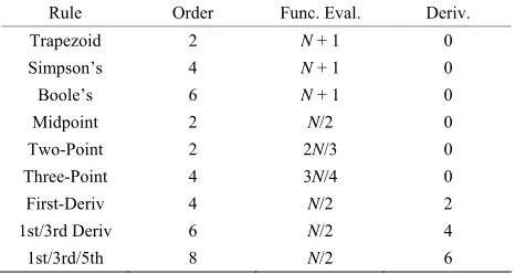
Table 3. Computational Cost for Closed and Open Newton- Cotes and Derivative-Based Quadrature Formula.
Rule Order Func. Eval. Deriv.
Trapezoid 2 N + 1 0
Simpson’s 4 N + 1 0
Boole’s 6 N + 1 0
Midpoint 2 N/2 0
Two-Point 2 2N/3 0
Three-Point 4 3N/4 0
First-Deriv 4 N/2 2
1st/3rd Deriv 6 N/2 4
[image:4.595.308.539.250.582.2] [image:4.595.307.540.610.734.2]4. Numerical Results
To demonstrate the accuracy of the new numerical inte- gration formula based on the inclusion of the derivative,
the values of 2 2 0
e x d x
and
3 2 0
e xsin 4 d x x
are esti-mated using the midpoint rule and the first three deriva- tive-based midpoint quadrature rules, dealing with the first derivative, the first and third derivatives and the first, third and fifth derivatives.
The calculation of the order of accuracy is obtained using the following approach. Let represent the numerical results using step size . The following for- mula is used to calculate the observed order of accuracy
, involving numerical results , and or
N h
Nh
N h p
N
2h
4h
4 2
ln 2
ln 2
N h N h
N h N h
p
(20)
The programming language REXX [10,11] was used to generate these numerical results, using 50 significant digits for the calculations.
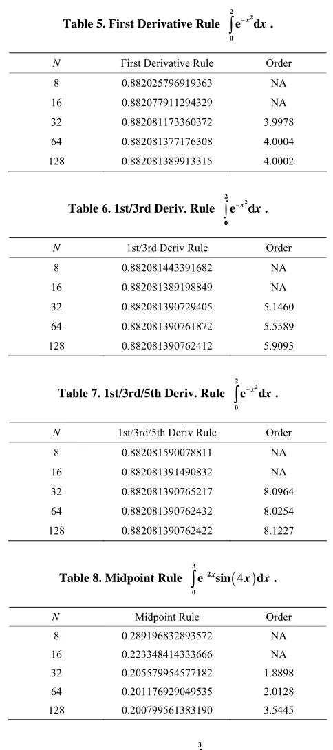
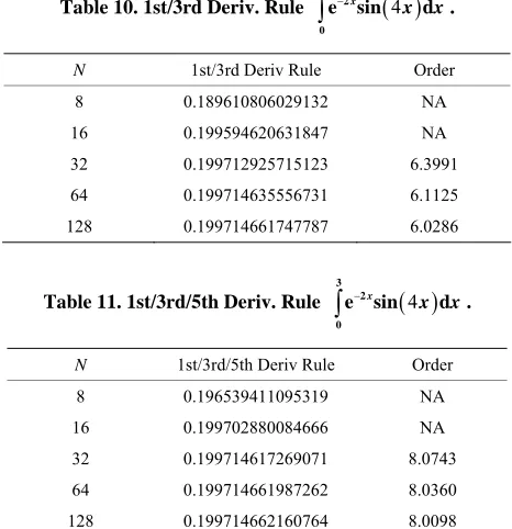
In Tables4-7, the results for the numerical approxima-
tion to 2 2 0
e x d x
are shown; and in Tables 8-11, the re-sults for the numerical approximation to
3 2 0
e xsin 4 d x x
are shown. For both integrals, the ob- served order of accuracy of the derivative-based mid- point quadrature formula is converging to the appropriate theoretical order of accuracy. The first derivative-based midpoint rule is clearly fourth order accurate; the first and third derivative rule is demonstrating sixth order accuracy; and the quadrature rule using first, third and fifth derivatives shows eighth order accurate results. For these methods, the derivatives are only evaluated at the overall endpoints of the interval of integration, rather than at the interior points. Thus, these methods are only slightly more computationally expensive than the mid- point rule, even though their accuracies are significantly higher.Table 4. Midpoint Rule
x . x 22
0
e d
N Midpoint Rule Order
8 0.882788948539727 NA 16 0.882268699199420 NA
32 0.882128870336645 1.8955
64 0.882093301420376 1.9750
[image:5.595.301.543.81.626.2]128 0.882084370974332 1.9938
Table 5. First Derivative Rule
x2 x.2
0
e d
N First Derivative Rule Order
8 0.882025796919363 NA 16 0.882077911294329 NA
32 0.882081173360372 3.9978
64 0.882081377176308 4.0004
128 0.882081389913315 4.0002
Table 6. 1st/3rd Deriv. Rule
x . x 22
0
e d
N 1st/3rd Deriv Rule Order
8 0.882081443391682 NA 16 0.882081389198849 NA
32 0.882081390729405 5.1460
64 0.882081390761872 5.5589
128 0.882081390762412 5.9093
Table 7. 1st/3rd/5th Deriv. Rule
x . x 22
0
e d
N 1st/3rd/5th Deriv Rule Order
8 0.882081590078811 NA 16 0.882081391490832 NA
32 0.882081390765217 8.0964
64 0.882081390762432 8.0254
128 0.882081390762422 8.1227
Table 8. Midpoint Rule
x
4 . x x3 2
0
e sin d
N Midpoint Rule Order
8 0.289196832893572 NA 16 0.223348414333666 NA
32 0.205579954577182 1.8898
64 0.201176929049535 2.0128
128 0.200799561383190 3.5445
Table 9. First Deriv. Rule
x
4 . x x3 2
0
e sin d
N 1st Deriv-Based Rule Order
8 0.195705275438686 NA 16 0.199975524969946 NA
32 0.199736732236252 4.1605
64 0.199716123464302 3.5344
These quadrature rules were obtained by using the concept of precision. If a quadrature rule has precision P, then it exactly integrates the monomials 1, x, through xP but not P1
[image:6.595.55.288.95.336.2]x . Using this concept, a system of P + 1 lin- ear equations in the coefficients of the quadrature for- mula can be generated. Furthermore, as is shown in the appendix, the concept of precision can be used to gener- ate the leading order error term for the quadrature for- mula.
Table 10. 1st/3rd Deriv. Rule
x
4x x.3 2
0
e sin d
N 1st/3rd Deriv Rule Order
8 0.189610806029132 NA 16 0.199594620631847 NA
32 0.199712925715123 6.3991
64 0.199714635556731 6.1125
128 0.199714661747787 6.0286
REFERENCES
Table 11. 1st/3rd/5th Deriv. Rule
x
4 .x x
3 2
0
e sin d [1] E. Babolian, M. Masjed-Jamei and M. R. Eslahchi, “On
Numerical Improvement of Gauss-Legendre Quadrature Rules,” Applied Mathematics and Computation, Vol. 160, No. 3, 2005, pp. 779-789. doi:10.1016/j.amc.2003.11.031
N 1st/3rd/5th Deriv Rule Order
8 0.196539411095319 NA 16 0.199702880084666 NA
32 0.199714617269071 8.0743
64 0.199714661987262 8.0360
128 0.199714662160764 8.0098
[2] M. R. Eslahchi, M. Masjed-Jamei and E. Babolian, “On Numerical Improvement of Gauss-Lobatto Quadrature Rules,” Applied Mathematics and Computation, Vol. 164,
No. 3, 2005, pp. 707-717. doi:10.1016/j.amc.2004.04.113
[3] M. R. Esclahchi, M. Dehghan and M. Masjed-Jamei, “On Numerical Improvement of the First Kind Gauss-Che- byshev Quadrature Rules,” Applied Mathematics and Computation, Vol. 165, No. 1, 2005, pp. 5-21.
doi:10.1016/j.amc.2004.06.102
5. Conclusions
New derivative-based midpoint quadrature rules were presented, along with their error terms. When using only odd derivatives, the coefficients for the odd derivatives sum to zero; thus, when using these quadrature rules in a composite formula, all of the derivatives at interior points cancel out. As a result, higher order accurate quadrature rules can be generated by only evaluating the odd deriva- tives at two locations, which are the endpoints of the in- terval of integration. These new derivative-based quad- rature rules are much more computationally efficient than the open and closed Newton-Cotes formula of the same order of accuracy. Additionally, these derivative-based midpoint quadrature rules build upon each other, so that the only change needed to increase the order of accuracy is to determine the coefficients (or weights) for the next odd derivative, without changing the weights for the lower odd derivatives.
[4] M. Dehghan, M. Masjed-Jamei and M. R. Eslahchi, “On Numerical Improvement of Closed Newton-Cotes Quad-rature Rules,” Applied Mathematics and Computation,
Vol. 165, No. 2, 2005, pp. 251-260.
doi:10.1016/j.amc.2004.07.009
[5] M. Masjed-Jamei, M. R. Eslahchi and M. Dehghan, “On Numerical Improvement of Gauss-Radau Quadrature Rules,” Applied Mathematics and Computation, Vol. 168,
No. 1, 2005, pp. 51-64. doi:10.1016/j.amc.2004.08.046
[6] M. R. Esclahchi, M. Dehghan and M. Masjed-Jamei, “The First Kind Chebyshev-Newton-Cotes Quadrature Rules (Closed Type) and Its Numerical Improvement,”
Applied Mathematics and Computation, Vol. 168, No. 1,
2005, pp. 479-495. doi:10.1016/j.amc.2004.09.048
[7] M. Dehghan, M. Masjed-Jamei and M. R. Eslahchi, “The Semi-Open Newton-Cotes Quadrature Rule and Its Nu-merical Improvement,” Applied Mathematics and Com-putation, Vol. 171, No. 2, 2005, pp. 1129-1140.
doi:10.1016/j.amc.2005.01.137 The computational cost for each of these methods was
analyzed and compared to both the open and the closed Newton-Cotes formula for two different integrals
[8] M. Dehghan, M. Masjed-Jamei and M. R. Eslahchi, “On Numerical Improvement of Open Newton-Cotes Quadra-ture Rules,” Applied Mathematics and Computation, Vol.
175, No. 1, 2006, pp. 618-627.
doi:10.1016/j.amc.2005.07.030
2 2 0
e x d x
and
3 2 0
e xsin 4 d x x
. The new derivative-based midpoint quadrature formula were superior com- putationally to the same order open or closed Newton- Cotes formula, primarily because of the computational efficiency of the midpoint rule, which only evaluates the function at half of the nodes, and the increase in the order of accuracy by evaluating the derivative at only two lo- cations.
[9] C. O. E. Burg, “Derivative-Based Closed Newton-Cotes Numerical Quadrature,” Applied Mathematics and Com-putation, Vol. 218, No. 13, 2012, pp. 7052-7065
doi:10.1016/j.amc.2011.12.060
[10] The REXX Language Association. http://www.rexxla.org
Appendix
In this appendix, a theorem concerning the leading order error term in a quadrature rule is proved. Based on its association with the Taylor Remainder Theorem, a con- jecture concerning the overall error term in a quadrature rule is made. A definition for a general quadrature rule of precision P is given below, followed by the theorem, its proof and the conjecture.
Definition: A numerical quadrature rule
approximates the integral
, , ,QR f x a b n
d ba f x x
using n uniformly spaced subintervals xi = a + ih where
h ba n to precision P if it exactly integrates the monomials 1, x, x2 through xP but not P1
x .
Theorem: Let f x
be infinitely differentiable on[a, b] and its Taylor series centered at x = a converges for all x
a b, . Let QR f x a b n
, , ,
be a quadra- ture rule of precision P. Then, the error between
d ba f x x
and approximation obtained by the quadra- ture rule is
1
d , , ,
d , , ,
! b a k b k k
k P a
f x x QR f x a b n
f a
x x QR x a b n
k
(21)Proof: This proof relies heavily on the Taylor series of
f x centered at xa, which is
0 0 1 ! ! k k k k P k kk k P
x a
f x f a
k
!
k
x a
f a f a
k
xka0 P
, 0 P (22)Since the quadrature rule exactly
integrates the monomials from x0 through xP, we know that
, , ,
QR f x a b n
d , , ,
b
k k
a
x x QR x a b n
(23)for all . By simple algebraic manipula- tions of lower order terms, it is obvious that
0,1, 2, ,
k
d
, ,b
k k
a
xa x QR xa a b n
(24)as well, for . Multiplying each equation by
0,1, 2, ,
k
k
f a and dividing by , the quadrature rule exactly integrates each of the first P + 1 terms in the Taylor series of
! k
f x , or
d
,! !
k k
b
k k
a
x a x a
f a x QR f a a b n
k k
, , 0
(25) for k0,1, , P. Thus,
0 0 0 0 1d , , ,
d !
, , , !
d , , ,
!
d , , ,
!
d , ,
! d ! b a k b k k a k k k k b k k a k b P k k k a k b k k
k P a
k
k
a
f x x QR f x a b n x a
f a x
k x a
QR f a a b n
k
f a
x a x QR x a a b n k
f a
x a x QR x a a b n k
f a
, x a x QR x a a b n k
f a
x a x
k
1 , , , b k k PQR x a a b n
(26)Note: the infinite summation can be interchanged with the definite integral, since the Taylor series converges for all values of x
a b, .Thus, the error term in the numerical quadrature rule approximation to the exact integral is an infinite Taylor series where the coefficients are determined from the monomials P1
x and higher. Because of this relation-ship to the Taylor series, the following conjecture is rea-sonable, since it follows the pattern observed in the infi-nite Taylor series and the Taylor polynomial with its remainder term. The error term obtained from this con-jecture agrees with the error terms for all quadrature formula that the author has studied.
Conjecture: Let f x
QRhave continuous de-rivatives on [a, b]. Let be a quadra-ture rule of precision P. Then, the error between
a
1
P
f x , , ,a b n
d bf x x
and approximation obtained by the quadra-ture rule is
1
1 1
d , , ,
, , , 1 ! b a P b P P a
f x x QR f x a b n f
x QR x a b n
P