Automatically designing more general mutation operators of evolutionary programming for groups of function classes using a hyper heuristic

Automatically Designing More General Mutation Operators

of Evolutionary Programming for Groups of Function

Classes Using a Hyper-Heuristic

Libin Hong

School of Computer Science

University of Nottingham P.R.C. [email protected]

John H. Drake

School of Computer Science

University of Nottingham P.R.C. [email protected]

John R. Woodward

Computing Science and Mathematics

University of Stirling U.K. [email protected]

Ender Özcan

Department of Computer Science

University of Nottingham U.K. [email protected]

ABSTRACT

In this study we use Genetic Programming (GP) as an offline hyper-heuristic to evolve a mutation operator for Evolution-ary Programming. This is done using the Gaussian and uniform distributions as the terminal set, and arithmetic operators as the function set. The mutation operators are automatically designed for a specific function class. The contribution of this paper is to show that a GP can not only automatically design a mutation operator for Evolutionary Programming (EP) on functions generated from a specific function class, but also can design more general mutation operators on functions generated from groups of function classes. In addition, the automatically designed mutation operators also show good performance on new functions gen-erated from a specific function class or a group of function classes.

Keywords

Hyper-Heuristic, Genetic Programming, Optimization, Func-tion Class

1.

INTRODUCTION

A hyper-heuristic searches for heuristics for computational search problems. During the searching process it can gener-ate or select heuristics according to its learning mechanism [4]. Burke et al. [5] proposed a distinction betweenonline

andofflinelearning, according to the source of the feedback during learning. For anonline hyper-heuristic, the learning occurs when the heuristic is solving an instance of a prob-lem. For anofflinehyper-heuristic collects knowledge, from a training a set of instances to solve unknown instances of the same problem. Recently GP has been used with

hyper-GECCO ’16, July 20-24, 2016, Denver, CO, USA

ACM ISBN 978-1-4503-2138-9. DOI:10.1145/1235

heuristics for the bin packing problem [6], the multidimen-sional knapsack problem [8], to evolve highly competitive general algorithms for envelope reduction in sparse matrices [12], to handle multiple conflicting objectives in dynamic job shop scheduling [18], to automatically design a mutation op-erator for Evolutionary Programming [10], to compare rule representations [11], to evolve due-date assignment models in job shop environments [20], to automatic design sched-ule policies for dynamic multi-objective job shop scheduling [19], to evolve ensembles of dispatching rules for the job shop scheduling problem [22], for feature selection and question– answer ranking in IBM Watson [2], to automated design production scheduling heuristics [3].

Burke et al. [6] proposed to automatically design heuris-tic for the bin packing problem and these heurisheuris-tics are “a Jack-of-all-Trades or a Master of One.” Burke et al. [6] point out that heuristics can be evolved to be specialists on a particular sub-problem, or general enough to work on all sub-problems. However there is a trade-off between per-formance and generalisation. The hypothesis of this paper, inspired by [6]: if the probability distribution over function instances is specific, we can design a specific EP mutation operator for a specific function class. We can also design a mutation operator of EP that performs well on a group of function classes. To verify this hypothesis we designed two types of experiment. In the first experiment, we tailor mutation operators for EP to a specific function class, and the best results are used as the fitness values for GP. This kind of experiment was proposed in [10]. In the second ex-periment, we tailor more general mutation operators for a group of function classes (each group contains three function classes) and use the number of outright wins as the fitness values for the GP. After completing the experiment, we test the Automatically Designed Mutation Operators (ADM) from both experiments and human designed mutation op-erators on a separate independent test set of functions. To make a fair comparison, we use Borda count to evaluate the performance. The comparison shows that the more general automatically designed mutation operators from the second experiment has the better performance on average on groups of function classes.

the training types and the parameter settings for GP and EP. In Section 4, we describe all the testing of ADMs on function classes to identify the performance of the result. In Section 5, we analyse and compare the testing results. In Section 6, we summarize and conclude the paper.

2.

FUNCTION OPTIMIZATION BY

EVOLU-TIONARY PROGRAMMING

EP is an algorithm to evolve a population of numerical vectors in order to find a global optimum of a function in a limited search region. Mutation is the only operator for EP. Researchers have made great efforts to finding and selecting mutation operators, or developing more advanced mutation strategies for EP in recent years [23, 24, 13, 7, 16, 15, 9].

Global minimization can be formalized as a pair (S, f), whereS∈Rnis a bounded set onRn andf:S−→Ris an n-dimensional real-valued function. Hence the EP algorithm searches for a global optimum within a limited space. The aim of EP is to find a pointxmin∈S such thatf(xmin) is

a global minimum onS. More specifically it is required to find anxmin∈S such that

∀x∈S:f(xmin)≤f(x)

Here f does not need to be continuous or differentiable but it must be bounded. The mutation process of EP can be represented by the following equations.

xi

0

(j) = xi(j) +ηi(j)Dj (1)

ηi

0

(j) =ηi(j)exp(γ

0

N(0,1) +γNj(0,1)) (2)

In the above equations, iis the dimension and j repre-sentsj−thcomponent of the vectors xi, xi0,ηiandηi0,Dj

represents the mutation operator, researchers usually use a Cauchy, Gaussian or L´evy distribution as the mutation op-erator [23, 24, 13]. For a complete description of EP, refer to [1]. Lee et al. [13] point out that the L´evy distribution with α=1.0 is the Cauchy distribution and with α=2.0 is the Gaussian distribution. We useα=1.0 andα=2.0 to rep-resent the Cauchy and Gaussian distribution. In this paper, the framework automatically designs a piece of the program for EP to replaceDj. Then the EP algorithm uses the

can-didate mutation operatorDj to do the training and testing

on functions generated from function classes.

3.

USING GP TO AUTOMATICALLY

DE-SIGN A MUTATION OPERATOR FOR EP

In this section we describe the methods that set up con-nections between GP and EP. The EP parameters we use for this paper are in Table 2. In order to reduce the time cost of the training phase, we set the number of generations for each function class, please refer to Section 3.3. The codes we list in Table 3 are implemented according to Mantegna’s description [17]. Equation 3 and 4 show how to generate a random variable from a L´evy distribution with the cor-respondingα (0.75≤ α≤ 1.95). In equation 3, V is cal-culated fromX and Y, where X is a random variant from aN(0, σ2) distribution and Y is a random variate from a

N(0,1) distribution. K(α) and C(α) are two parameters with real values, which can be looked up in [17], and must be determined properly. The values ofσx,K(α) andC(α)

used in this paper are listed in Table 4. For a more detailed derivation of the equations, please refer to [17].

V = X

|Y |1/α (3)

W = ((K(α)−1)exp(−V /C(α)) + 1)V (4)

3.1

Functions and Function Classes

In a suite of 23 functions often used in EP research [23, 24], the functions can be classified as: f1–f7 are unimodal functions,f8–f13are multimodal functions with many local optima, f14–f23 are multimodal functions with a few local optima [24].

In this study, we do not use single functions for benchmark function optimisation. Instead, we use function classes, where each class is a single parameterised function which embodies a set of unique functions each having fixed parameter val-ues. Based on these 23 functions, we have constructed corre-sponding function classes. To distinguish between functions and function classes, we use the notation fg to represent

function andFg to represent function class. In this paper,

we select 3 function classes from each of the unimodal, and multimodal with many and few local optima (F1, F2, F6,

F10, F12, F13, F16, F19 and F23). The training and test function classes used in this study are given in Table 1, with the index of each function class corresponding to the origi-nal functions of [23]. In Table 1,ai,bi andci are uniformly

distributed in range [1,2], [−1,1] and [−1,1], respectively. An example of a function class is: y =Pn

i=1aix 2

i, in this

casey=Pn i=11.3x

2

i is a function from this function class,

whiley=Pn i=10.3x

2

i is not from this function class.

3.2

Experimental Design and Fitness Functions

for GP

The experiments can be divided into two different training types: one type of training is for a specific function class, e.g.,F1, another type of training is for a group of function classes, e.g., the unimodalF1,F2 andF6. We designed two different fitness functions for each training. In both training types the GP settings are the same, only the functions vary. For the parameter settings of GP, please refer to Table 5. We call a program generated by GP an Automatically Designed Mutation operator (ADM). The tailored ADM automati-cally designed for a function classFg by training type 1 is

represented by ADMg, wheregis the function class index.

ADMgis called a dedicated ADM for function classFg. The

tailored ADM automatically designed for a group of func-tion classesFg,FjandFkby training type 2 is represented

asADMg,j,k, whereg,j,krepresent the indexes of the

dif-ferent function classes. ADMg,j,k is called a more general

ADM for function class on Fg,Fj andFk. To distinguish

the fitness functions for each type of training, we describe training of type 1 and training of type 2 in the paragraphs below.

Training Type 1: EachADMg is used as an EP

mu-tation operator on 9 functions drawn from a given function class. The fitness of an ADMg is the average of the best

[image:3.612.109.503.69.368.2]

Table 1 Function Classes withndimensions and domainS,ai∈[1,2],bi, ci∈[−1,1].

F unction Class n S

F1 (x) =Pn

i=1[(aixi−bi)2 +ci] 30 [−100,100]n

F2 (x) =Pn

i=1|aixi|+

Qn

i=1|bixi| 30 [−10,10]n

F3 (x) =Pn i=1[ai

Pi

j=1xj]2 30 [−100,100]n

F4 (x) = max_i{|aixi|,1≤i≤n} 30 [−100,100]n

F5 (x) =Pn

i=1[ai(xi+1−x2_i)2 +bi(xi−1)2 +ci] 30 [−30,30]n

F6 (x) =Pn

i=1(baixi+ 0.5c)2 +bi 30 [−100,100]n

F_{7 (}x) =Pn

i=1aiix4i+random[0,1) 30 [−1.28,1.28]n

F_{8 (}x) =Pn

i=1−(xisin(

p

|xi|) +ai) 30 [−500,500]n

F9 (x) =Pn

i=1[aix2i+bi(1−cos(2πxi))] 30 [−5.12,5.12]n F_{10 (}x) =−exp(−0.2q1_nPn

i=1aix2i)−exp( 1n Pn

i=1bicos 2πxi) +e 30 [−32,32]n

F11 (x) =₄₀₀₀ai Pn i=1x2i−bi

Qn

i=1cos(xi√_i) 30 [−600,600]n

F12 (x) =π_n{10sin2 (πyi) +aiPn−1

i=1(yi−1)2 [1 + 10sin2 (πyi+1 ) + (yn−1)2 ]}+Pn

i=1u(xi,10,100,4),

yi= 1 + 1₄(xi+ 1)

u(xi, w, k, m) =

  

k(xi−w)m , xi > w,

0, −w≤_xi≤w, k(−_xi−w)m , xi <−w.

30 [−50,50]n

F_{13 (}x) = 0.1{sin2 (3πx_{1 ) +}aiPn−1

i=1(xi−1)2 [1 +sin2 (3πxi+1 )] + (xn−1)[1 +sin2 (2πxn)]}+Pn

i=1u(xi,5,100,4)

30 [−50,50]n

F14 (x) = [₅₀₀1 +aiP25

i=1_j+P2 1

i=1(xi−wij)6

]−1 2 [−65.536,65.536]n

F15 (x) =P11

i=1[wi−

aix1 (y2i+yix2 )

bi(y2

i+yix3 +x4 )

]2 4 [−5,5]n

F16 (x) =a1 (4x2₁−2.1x4_{1 +}1₃x6_{1 +}x1x2−4x2_{2 + 4}x_{2 ) +}4 b1 2 [−5,5]n

F17 (x) =a1 (x2−₄5_π.12x21 +5πx1−6)2 + 10b1 (1−81π)cosx1 + 10 2 [−5,10]×[0,15]

F18 (x) =a1 [1 + (x1 +x2 + 1)2 (19−14x1 + 3x2₁−14x2 + 6x1x2 + 3x2_{2 )]}×[30 + (2x1−3x2 )2 (18−32x1 + 12x2_{1 + 48}x₂−36x₁x_{2 + 27}x2_{2 )] +}b₁

2 [−2,2]n

F_{19 (}x) =−P4

i=1yiexp[−

P4

j=1aj wij(xj−pij)2 +bi] 3 [0,1]n

F20 (x) =−P4

i=1yiexp[−

P6

j=1aj wij(xj−pij)2 +bi] 6 [0,1]n

F21 (x) =−P5

i=1ai[(x−wi)T(x−wi) +yi+bi]−1 4 [0,10]n

F22 (x) =−P7

i=1ai[(x−wi)T(x−wi) +yi+bi]−1 4 [0,10]n

F23 (x) =−P10

[image:3.612.364.519.434.675.2]

i=1ai[(x−wi)T(x−wi) +yi+bi]−1where yi= 0.1 4 [0,10]n

Table 2 Parameter settings for EP.

Parameter Settings

population size 100

tournament size 10

[image:3.612.70.304.438.476.2]

initial standard deviations of initial population 3.0

Table 3 How the L´evy distribution is constructed from the normal distribution.

Algorithm for L´evy distribution

α1 = 1.0/α X=N(0, σ2)

Y =N(0,1)

V =X/(abs(Y)α1)

W= ((K(α)−1)∗exp(−abs(V)/C(α)) + 1.0)∗V

Table 4αvalues and relatedσ2,K(α) andC(α).

α σ2 K(α) C(α) 1.2 0.878829 1.20519 2.941 1.4 0.759679 1.44647 2.8315 1.6 0.628231 1.79361 2.6125 1.8 0.458638 2.50147 2.206

Table 5 Parameter settings for GP.

Parameter Settings

crossover proportion 45%

mutation proportion 45%

reproduction proportion 10%

selection method lexictour [14]

tournament size 2

depthnodes 2 [14]

population size 20

maximum generation 25

elitism keep best

Table 6 Function set for GP.

Symbol Function Arity

+ addition 2

− subtraction 2

× multiplication 2

÷ protected division 2

power power 2

exp exponential function 1

abs absolute 1

Table 7 Terminal set for GP.

Symbol Terminal

N(µ, σ2) Normal Distribution

[image:3.612.89.283.515.568.2]

This type of training was used in [10]. In this training, the fitness value of the GP is from the averaged fitness values of 9 EP runs.

Training Type 2: We train ADMg,j,k on 9 functions

(three from each ofFg,FjandFk) by GP. Then we validate

ADMg,j,kon 9 separate functions (three from each ofFg,Fj

andFk). If the fitness value of the EP that usesADMg,j,k

beats all of the human designed mutation operators (L´evy distribution (withα=1.0, 1.2, 1.4, 1.6, 1.8, 2.0)), L´evy with

α= 1.0 is Cauchy, L´evy withα= 2.0 is Gaussian), on the given function, it scores 1 point, thus it can score between 0 and a maximum of 9 (we call this the number of outright wins). Here we use the number of outright wins because averaging fitness values can be skewed by a single large value, and using a rank-based method is more robust to outliers. In this training, the fitness value of the GP is the number of outright wins.

For both training types, the framework can not only ex-press a number of currently existing human designed EP mu-tation operators (Cauchy, Gaussian and L´evy distributions), but also can generate new kinds of mutation operators for EP. The main aim of this paper is to set up an algorithmic framework which can automatically design a more general mutation operator for EP on groups of function classes. We use GP as anoffline hyper-heuristic to evolve a mutation operator for EP. But in contrast to what we have done in [10], in this paper the hyper-heuristic uses three groups of function classes, each group containing three function classes

Fg,FjandFk, whereg,j,kare different indexes of function

classes.

3.3

Parameter Settings for EP

The settings for EP are presented in Table 2: the pop-ulation size is set to 100, the tournament size is set to 10, the initial standard deviations is set to 3.0. The settings for dimensionsnand domainsSare listed in Table 1. We have to point out that in our experiment the maximum number of generations of EP is set to 1000 forF1,F2,F6,F10,F12

andF13. The maximum number of generations of EP is set to 100 forF16,F19andF23.

3.4

Parameter Settings for GP

The parameter settings for GP are listed in Table 5. The function set and terminal set of GP are listed in Table 6 and 7. µ is a random number in [−2,2], as we wish the designed mutation operator is not Y-axis symmetric. σ2 _is

a random number in [0,5]. depthnodesis set as 2 indicates restrictions are to be applied in tree size (number of nodes) [14]. U is the uniform distribution with range [0,3]. The other settings of GP are: population size 20, the maximum number of generations 25. The settings of GP in Table 5 are able to generate the values in Table 4, and the (human designed) piece of programs in Table 3 and other programs.

4.

TESTING AUTOMATICALLY DESIGNED

MUTATION OPERATORS

We employADM s(in Table 14) and human designed mu-tation operators on EP and test them on each function class

Fg. For eachADMwe record 50 values from 50 independent

EP runs, each being the lowest value through all generations of EP, we then average them, this is called the mean best values. We test allADMs onFg respectively. In all

test-ing the generated functions from each function class are the

same. This means the results in Tables 8, 9, 10, 11, 12 and 13 are based on the same 50 functions generated from each function classFg.

4.1

Testing the More General ADMs and

Hu-man Designed Mutation Operators

We did the testing forADMg,j,kand human designed

mu-tation operators (L´evy distribution (with α=1.0, 1.2, 1.4, 1.6, 1.8, 2.0)) on Fg. The mean best values and standard

deviations are listed in Table 8. Based on the original data for Table 8, we also calculate the Borda countsBgfor all test

mutation operators to compare the performance ofADM1,2,6,

ADM10,12,13, ADM16,19,23 and human designed mutation

operators (in all, 9 mutation operators) in Table 10. We follow the method to calculate Borda counts in [21]: Test each mutation operator for each function and it has a rank

Rmn, wheremis the function index (1≤m≤50) andnis

the mutation operator index (1≤n≤9). The value ofRmn

is in range [1, 9]. The Borda counts Bg =Pm_i=1Rmn(m∈

1,2,3, ...50), is the sum of Rmn on 50 functions generated

from the function classFg; it has its best possible value 50

and the worst possible value 450 (gis the index of the func-tion class). Each mutafunc-tion operator has Borda countsBgon

Fg and the sum of the Borda countsBg,j,k=Bg+Bj+Bk.

4.2

Testing More General ADMs and

Dedi-cated ADMs

To observe the performance of dedicatedADMgandADMg,j,k

onFg, we testedADMg and ADMg,j,k onFg. We list the

mean best values and standard deviations in Table 11. In this table we consolidate the mean best values and standard deviations forADM1,2,6,ADM10,12,13andADM16,19,23, we

also put more decimal places forF16andF19, as otherwise, the results are too close to distinguish. We use the Borda counts to compare the performance of the 12 mutation op-erators in Table 13. In this comparison, the number of func-tionsp= 50 and the number of mutation operatorsq= 12. Therefore, the best possible score is 50, and the worst pos-sible is 600. Each mutation operator has Borda counts Bg

onFg, each mutation operator has the sum of Borda counts

Bg,j,k=Bg+Bj+Bk.

4.3

Testing More General ADMs and Human

Designed Mutation Operators on Non-Trained

Function Classes

To observe the performance ofADMg,j,kon Non-Trained

Function Classes (F3,F4,F5,F7,F8,F9,F11,F14,F15,F17,

F18, F20, F21 and F22), we tested ADMg,j,k and human

designed mutation operators (L´evy (α =1.0, 1.2, 1.4, 1.6, 1.8, 2.0)) on Non-Trained Function Classes. The results are in Table 15.

5.

ANALYSIS AND COMPARISON

In this section we compare the mutation operatorsADMg,j,k,

ADMg and the human designed mutation operators. An

ADMgdesigned for the function classFgis called a tailored

mutation operator, while an ADMg tested on Fj is called

a non-tailored mutation operator. For example, ADM1 is tailored mutation operator for F1, but it is a non-tailored mutation operator for the function classF2. Similarly for a group of function classesF1,F2andF6,ADM1,2,6is a more

func-tion classes, while ADM10,12,13 and ADM16,19,23 are

non-tailored mutation operators.

5.1

Analysis and Comparison of More

Gen-eral ADMs and Human Designed

Muta-tion Operators

From Table 8, 9, 11 and 12 we can see that ADMg,j,k

show the outstanding performance on allFg in most cases.

In Table 10, which presents the Borda counts, among all Borda counts of tested mutation operators, ADMg,j,k has

the best/lowest scores on the groups of function classes: the Borda counts B1,2,6 of ADM1,2,6 is 344, which is the

best/lowest value on F1, F2 and F6. The Borda counts

B10,12,13 of ADM10,12,13 is 320, which is the best/lowest

value on F10, F12 and F13. The Borda counts B16,19,23 of

ADM16,19,23 is 213, which is the best/lowest value onF16,

F19 and F23. AlthoughB1, B2 and B6 forADM1,2,6 are

not the best values for F1, F2 and F6, B1,2,6 the sum of B1, B2 and B6 shows that ADM1,2,6 has the best

perfor-mance among all tested mutation operators. B12 and B13

forADM10,12,13 are the best/lowest value on F12 and F13

respectively, B10 of ADM1,2,6 show the best performance

onF10. We think this is because the function characteris-tics ofF10are different from the characteristics ofF12 and

F13. B16,B19 andB23forADM16,19,23 are the best/lowest

value onF16,F19andF23respectively. In general, a tailored

ADMg,j,k always show a better performance than the

hu-man designed mutation operator and non-tailoredADMg,j,k.

Table 9 shows the results of the Wilcoxon Signed-Rank Test within 5% significance level comparing a tailoredADMg,j,k

compared with human designed mutation operators (L´evy distribution (withα=1.0, 1.2, 1.4, 1.6, 1.8, 2.0)). Table 12 shows the results of a Wilcoxon Signed-Rank Test within 5% significance level comparing a tailoredADMg,j,k compared

with otherADMs. In both tables, “≥” and “≤” indicate that theADMg,j,kperforms better or worse onFg,FjandFk

re-spectively, compared to human designed mutation operators or ADMs. In the case that this difference is statistically sig-nificant, “>” and “<” are used.

5.2

Analysis and Comparison of More

Gen-eral ADMs and ADMs

In Table 11 the results using ADMg to do test on Fg.

ADM1,ADM2,ADM6,ADM12,ADM19andADM23show

the best performance onF1,F2,F6,F12,F19andF23 respec-tively. ADM10shows the second best performance on F10, asADM1,2,6 has the best performance onF10. ADM13has

the third best performance onF13, asADM12andADM10,12,13

beatADM13onF13. ADM16is a special case,ADM16does

not show any outstanding performance among theADMs on

F16. We think this is because the training of ADM16 was insufficient, or we need to record more decimals to do the analysis, as the values inboldfaceare the same.

In Table 13 the Borda counts B1,2,6 of ADM1,2,6 is 434,

which beats all otherADMs onF1,F2 andF6. The Borda countsB10,12,13ofADM10,12,13is 441, which beats all other ADMs onF10, F12 and F13 as well. However, the Borda counts B16,19,23 of ADM16,19,23, which is the second best

value, is 393 on F16, F19 and F23. The best value 284 is that of the Borda countsB16,19,23 of ADM19 onF16, F19

and F23. This is an acceptable exception, as in the GP training system we only use the human designed mutation operator to evaluate the performance of the ADMs, both

ADMg and ADMg,j,k beat the human designed mutation

operator separately.

Overall, the results in Table 11 and 13 demonstrate that the tailored mutation operatorADMghas better mean best

values than the non-tailored mutation operators andADMg,j,k

on Fg, although there are some exceptions (for example,

ADM10onF10andADM16 onF16are not the best). The

Borda counts in Table 13 demonstrate that the tailored gen-eral mutation operatorADMg,j,khas better performance on

the groups of function classesFg,FjandFk. BothADMg,j,k

and ADMg have better performances than the human

de-signed mutation operators on average; the experiment we designed successfully found a more general mutation opera-torADMg,j,k that has better performance than other

mu-tation operators on a group of function classes Fg, Fj, Fk

on average.

5.3

Analysis and Comparison of More

Gen-eral ADMs and Human Designed

Muta-tion Operators on Non-Trained FuncMuta-tion

Classes

In Table 15, we test the more general mutation operator

ADMg,j,k and the human designed mutation operators on

the non-trained function classesFg over 50 runs. From this

table, although ADM1,2,6 does not show the best

perfor-mance onF3,F4,F5,F7, its performance is not the worst, we think this is because ADM1,2,6 fit F1,F2 and F6 well,

but may have over-fit on F3, F4,F5 andF7. ADM10,12,13

show the best performance on F8, and the second best on

F9,F11.ADM16,19,23has the best performance onF17,F18,

F20, F21, F22, but has the worst performance on F14 and

F15, we think this is becauseF14andF15has different func-tion characteristics, and henceADM10,12,13cannot fit them

well.

To make the results can be easily observed. In Table 8 and 15 the mean best values are in bold. In Table 9 and 12 “>” are in bold. In Table 10 and 13 the lowest Borda countsBg andBg,j,kof the tested mutation operator are in

bold. In Table 11 the mean best values usingADMg to do

test onFg are inboldand the results which are lower than

test result ofADMg onFg are also inbold.

6.

SUMMARY AND CONCLUSIONS

In this paper we designed a framework to automatically design more general tailored mutation operators for several groups of function classes. Previously, researchers have used GP to tailor mutation operators [10] for EP on a specific function class. We proposed using the number of outright wins, the number of times that automatically designed mu-tation operator has beaten the human designed mumu-tation operators, as the fitness value for the GP. We did the test to evaluate the performance of the more general tailored mu-tation operators, tailored mumu-tation operators and human designed mutation operators on a specific function class and on groups of function classes.

group of function classes. Thirdly, both tailored mutation operator and more general tailored mutation operator have better performances than human designed mutation oper-ators. Fourthly, compared with the more general tailored mutation operator and the tailored mutation operator on a specific function class, tailored mutation operator usually has better performance on a specific function class, but the more general tailored mutation operator usually has better performance on a group of function classes on average.

7.

REFERENCES

[1] T. Back and H.-P. Schwefel. An overview of evolutionary algorithms for parameter optimization.

Evolutionary Computation, 1:1–23, 1993.

[2] U. Bhowan and D. McCloskey. Genetic programming for feature selection and question-answer ranking in ibm watson. InGenetic Programming, volume 9025 of

Lecture Notes in Computer Science, pages 153–166. Springer International Publishing, 2015.

[3] J. Branke, S. Nguyen, C. W. Pickardt, and M. Zhang. Automated design of production scheduling heuristics: A review.IEEE Transactions on Evolutionary Computation, 20(1):110–124, Feb 2016.

[4] E. K. Burke, M. Gendreau, M. Hyde, G. Kendall, G. Ochoa, E. ¨Ozcan, and R. Qu. Hyper-heuristics: A survey of the state of the art.Journal of the

Operational Research Society, pages 1695–1724, 2013. [5] E. K. Burke, M. Hyde, G. Kendall, G. Ochoa,

E. ¨Ozcan, and J. R. Woodward. A classification of hyper-heuristic approaches. InHandbook of Metaheuristics, pages 449–468. Springer US, 2010. [6] E. K. Burke, M. R. Hyde, G. Kendall, and

J. Woodward. Automatic heuristic generation with genetic programming: evolving a jack-of-all-trades or a master of one. InProceedings of the 9th Annual Conference on Genetic and Evolutionary

Computation, pages 1559–1565. 2007.

[7] H. Dong, J. He, H. Huang, and W. Hou. Evolutionary programming using a mixed mutation strategy.

Information Sciences, 177(1):312–327, 2007. [8] J. H. Drake, M. Hyde, K. Ibrahim, and E. ¨Ozcan. A

genetic programming hyper-heuristic for the multidimensional knapsack problem. 43:1500–1511, 2014.

[9] L. Hong, J. H. Drake, and E. ¨Ozcan. A step size based self-adaptive mutation operator for evolutionary programming. InProceedings of Genetic and Evolutionary Computation Conference 2014, pages 1381–1388. ACM, 2014.

[10] L. Hong, J. Woodward, J. Li, and E. ¨Ozcan. Automated design of probability distributions as mutation operators for evolutionary programming using genetic programming. InGenetic Programming, volume 7831 ofLecture Notes in Computer Science, pages 85–96. Springer Berlin Heidelberg, 2013. [11] T. H. J. Branke and B. Scholz-Reiter. Hyper-heuristic

evolution of dispatching rules: A comparison of rule representations. volume 23, pages 249–277.

Evolutionary Computation, 2014.

[12] B. Koohestani and R. Poli. A genetic programming approach for evolving highly-competitive general algorithms for envelope reduction in sparse matrices.

InProceedings of the 12th International Conference on Parallel Problem Solving from Nature, volume 2, pages 287–296. Springer-Verlag, Berlin, Heidelberg, 2012. [13] C.-Y. Lee and X. Yao. Evolutionary programming

using mutations based on the l´evy probability distribution.IEEE Transactions on Evolutionary Computation, 8(1):1–13, 2004.

[14] S. Luke and L. Panait. Lexicographic parsimony pressure. InProceedings of Genetic and Evolutionary Computation Conference 2002, pages 829–836. Morgan Kaufmann Publishers, 2002.

[15] R. Mallipeddi, S. Mallipeddi, and P. Suganthan. Ensemble strategies with adaptive evolutionary programming.Information Sciences,

180(9):1571–1581, 2010.

[16] R. Mallipeddi and P. N. Suganthan. Evaluation of novel adaptive evolutionary programming on four constraint handling techniques. InProceedings of IEEE World Congress on Computational Intelligence, pages 4045–4052. 2008.

[17] R. N. Mantegna. Fast, accurate algorithm for numerical simulation of l´evy stable stochastic

processes.Physical Review E, 49:4677–4683, May 1994. [18] S. Nguyen, M. Zhang, M. Johnston, and K. Tan.

Dynamic multi-objective job shop scheduling: A genetic programming approach. InAutomated Scheduling and Planning, volume 505 ofStudies in Computational Intelligence, pages 251–282. Springer Berlin Heidelberg, 2013.

[19] S. Nguyen, M. Zhang, M. Johnston, and K. C. Tan. Automatic design of scheduling policies for dynamic multi-objective job shop scheduling via cooperative coevolution genetic programming.IEEE Transactions on Evolutionary Computation, 18(2):193–208, April 2014.

[20] S. Nguyen, M. Zhang, M. Johnston, and K. C. Tan. Genetic programming for evolving due-date assignment models in job shop environments.

Evolutionary Computation, 22(1):105–138, March 2014.

[21] G. Ochoa, J. Walker, M. Hyde, and T. Curtois. Adaptive evolutionary algorithms and extensions to the hyflex hyper-heuristic framework. InProceedings of Parallel Problem Solving from Nature - PPSN XII: 12th International Conference, volume 7492 ofLecture Notes in Computer Science, pages 418–427. Springer Berlin Heidelberg, 2012.

[22] J. Park, S. Nguyen, M. Zhang, and M. Johnston. Evolving ensembles of dispatching rules using genetic programming for job shop scheduling. InGenetic Programming, volume 9025 ofLecture Notes in Computer Science, pages 92–104. Springer International Publishing, 2015.

[23] X. Yao and Y. Liu. Fast evolutionary programming. In

Proceedings of the 5th Annual Conference on Evolutionary Programming, pages 451–460. MIT Press, 1996.

[image:7.612.119.697.82.249.2]

Table 8 The results ofADMg,j,k, L´evy(1.0, 1.2, 1.4, 1.6, 1.8, 2.0) on trained function classesFg. Mean indicates the mean of the best values found over all generations

over 50 runs forFg. Std Dev stands for standard deviations.

Fg ADM1,2,6 ADM10,12,13 ADM16,19,23 α= 1.0 α= 1.2 α= 1.4 α= 1.6 α= 1.8 α= 2.0

F1

Mean 0.3711 0.3624 166.2 0.3624 0.3654 0.3797 0.5124 0.5567 1.0003

Std Dev (3.11) (3.19) (883.8) (3.19) (3.19) (3.19) (3.17) (3.12) (3.25)

F2 _{Std Dev}Mean _(4.40E-03)0.040 _(9.16E-03)0.072 _(9.59E-02)0.043 _(1.48E-02)0.160 _(1.42E-02)0.109 _(9.03E-03)0.089 _(8.54E-03)0.077 _(6.13E-03)0.068 _(6.51E-03)0.048

F6

Mean 0.50 0.46 729.1 0.46 0.52 1.48 178.5 111.4 605.9

Std Dev (3.41) (3.41) (1621.6) (3.41) (3.49) (5.92) (1179.3) (312.1) (1578.1)

F10

Mean -20.04 -19.24 -7.77 -3.66 -15.58 -19.05 -17.32 -14.32 -10.71

Std Dev (0.31) (3.86) (5.93) (7.58) (8.24) (2.78) (2.52) (3.99) (4.09)

F12 _{Std Dev}Mean 0.0148_(0.03) 0.0031_(0.02) 3.1889_(2.91) 0.0135_(0.05) 0.1117_(0.20) 0.7234_(1.00) 1.1435_(1.14) 2.2114_(1.88) 4.0837_(3.85)

F13

Mean 0.0936 0.0042 20.85 0.0074 0.4746 4.10 12.42 14.21 27.54

Std Dev (0.24) (0.01) (25.4) (0.02) (1.52) (10.2) (12.9) (19.9) (28.3)

F16

Mean -1.803489196 -1.803489196 -1.803489196 -1.80348918 -1.803489185 -1.803489184 -1.803489186 -1.803489186 -1.803489192

Std Dev (0.65) (0.65) (0.65) (0.65) (0.65) (0.65) (0.65) (0.65) (0.65)

F19 _{Std Dev}Mean -5.23096752_(1.99) -5.230967433_(1.99) -5.230967576_(1.99) -5.225685243_(1.99) -5.225723116_(1.98) -5.230937535_(1.99) -5.225024015_(1.99) -5.225726632_(1.98) -5.230966751_(1.99)

F23

Mean -1.55E+07 -1.83E+07 -9.75E+07 -1.33E+06 -3.78E+06 -7.60E+06 -3.10E+06 -6.41E+06 -3.50E+06

[image:7.612.175.639.292.386.2]

Std Dev (4.22E+07) (7.02E+07) (3.26E+08) (2.46E+06) (1.19E+07) (2.62E+07) (6.94E+06) (2.61E+07) (5.76E+06)

Table 9 Wilcoxon Signed-Rank Test ofADMg,j,kversus L´evy Distribution (withα= 1.0, 1.2, 1.4, 1.6, 1.8, 2.0).

Fg ADMg,j,k ADM1,2,6 ADM10,12,13 ADM16,19,23 α= 1.0 α= 1.2 α= 1.4 α= 1.6 α= 1.8 α= 2.0

F1 ADM1,2,6 N/A < > < ≤ ≥ > > >

F2 ADM1,2,6 N/A > > > > > > > >

F6 ADM1,2,6 N/A = > = = > > > >

F10 ADM10,12,13 > N/A > > > > > > >

F12 ADM10,12,13 > N/A > ≥ > > > > >

F13 ADM10,12,13 > N/A > ≥ > > > > >

F16 ADM16,19,23 = = N/A > > > > > ≥

F19 ADM16,19,23 > > N/A > > > > > >

F23 ADM16,19,23 ≥ ≥ N/A > ≥ ≥ ≥ > >

Table 10 Borda counts for differentADM sonFg.

Fg Bg/Bg,j,k ADM1,2,6 ADM10,12,13 ADM16,19,23 α= 1.0 α= 1.2 α= 1.4 α= 1.6 α= 1.8 α= 2.0

F1 B1 187 125 447 154 167 195 293 312 370

F2 B2 99 241 95 447 388 343 276 225 136

F6 B6 58 50 408 50 57 129 280 336 404

F1F2F6 B1,2,6 344 416 950 651 612 667 849 873 910

F10 B10 72 122 364 403 214 182 246 300 347

F12 B12 134 105 380 116 192 260 313 357 393

F13 B13 157 93 376 104 184 250 347 352 387

F10F12F13 B10,12,13 363 320 1120 623 590 692 906 1009 1127

F16 B16 55 55 50 267 247 228 222 221 130

F19 B19 110 140 50 354 344 345 340 312 245

F23 B23 184 207 113 346 305 270 286 270 269

[image:7.612.168.648.428.547.2]

[image:8.612.73.776.71.239.2]

Table 11 The means and standard deviations for differentADM stested on different function classes.

Fg ADM1,2,6 ADM10,12,13 ADM16,19,23 ADM1 ADM2 ADM6 ADM10 ADM12 ADM13 ADM16 ADM19 ADM23

F1

Mean 0.3711 0.3624 166.2 0.3622 1.5873 0.3951 0.6019 0.3630 0.3625 3553.7 17432.0 54819.6

Std Dev (3.11) (3.19) (883.8) (3.19) (3.43) (3.18) (3.25) (3.19) (3.19) (2653.7) (8861.4) (12936.5)

F2

Mean 0.040 0.072 0.043 0.085 0.034 0.383 0.035 0.136 0.081 15.48 44.78 94.83

Std Dev (4.40E-03) (9.16E-03) (9.59E-02) (1.11E-02) (7.12E-03) (9.87E-02) (5.42E-03) (1.77E-02) (1.15E-02) (5.94) (11.87) (13.41)

F6 Mean_{Std Dev (3.41)}0.50 0.46_(3.41) 729.1_{(1621.6) (3.41)}0.46 1759.5_{(3887.0) (3.41)}0.46 _(5.42)2.86 0.46_{(3.41) (3.41)}0.46 _(7885.0)12656.2 _(15600.2)33359.4 84031.8_(22680.6)

F10

Mean -20.04 -19.24 -7.77 -20.03 -10.26 -0.47 -19.67 -12.04 -17.23 -3.22 -0.46 -0.74

Std Dev (0.31) (3.86) (5.93) (0.31) (3.11) (2.78) (0.85) (9.72) (6.92) (1.82) (0.32) (0.48)

F12

Mean 0.0148 0.0031 3.1889 0.0018 4.9436 0.0475 0.4014 0.0025 0.0031 79742.8 9159012.9 187046819.3

Std Dev (0.03) (0.02) (2.91) (0.01) (3.32) (0.12) (0.71) (0.02) (0.01) (157289.1) (12782055.1) (78867738.0)

F13 Mean_{Std Dev (0.24)}0.0936 0.0042_(0.01) 20.85_{(25.4) (0.06)}0.0172 26.99_{(27.2) (0.19)}0.0972 _(2.02)0.8932 0.0036_{(0.01) (0.01)}0.0054 _(28202.4)17023.8 _(10250182.6)7383897.8 217114903.0_(80527486.2)

F16

Mean -1.803489196 -1.803489196 -1.803489196-1.803489194 -1.803489194 -1.803489191 -1.803489196-1.803489194 -1.803489196 -1.803489195 -1.803489196-1.767501128

Std Dev (0.65) (0.65) (0.65) (0.65) (0.65) (0.65) (0.65) (0.65) (0.65) (0.65) (0.65) (0.65)

F19

Mean -5.23096752 -5.230967433 -5.230967576 -5.230967286 -5.22617391 -5.221829996 -5.230967563 -5.230794029 -5.230967504 -5.23096744 -5.230967578-4.966909097

Std Dev (1.99) (1.99) (1.99) (1.99) (1.99) (1.99) (1.99) (1.99) (1.99) (1.99) (1.99) (1.91)

[image:8.612.119.695.281.376.2]

F23 Mean_{Std Dev (4.22E+07)}-1.55E+07 -1.83E+07_(7.02E+07) -9.75E+07_{(3.26E+08) (1.81E+07)}-9.24E+06 -3.20E+07_{(1.54E+08) (7.97E+07)}-1.55E+07 _(1.67E+08)-5.10E+07 -7.03E+06_{(2.72E+07) (4.11E+07)}-1.12E+07 _(2.67E+07)-1.34E+07 _(9.05E+08)-4.27E+08 -3.86E+10_(2.49E+11)

Table 12 Statistically significant (Wilcoxon) comparison of differentADM s.

Fg ADMg,j,k ADM1,2,6 ADM10,12,13 ADM16,19,23 ADM1 ADM2 ADM6 ADM10 ADM12 ADM13 ADM16 ADM19 ADM23

F1 ADM1,2,6 N/A < > < > > > < < > > >

F2 ADM1,2,6 N/A > > > > > < > > > > >

F6 ADM1,2,6 N/A = > = > = > = = > > >

F10 ADM10,12,13 < N/A > ≤ > > < > > > > >

F12 ADM10,12,13 > N/A > ≤ > > > ≤ ≤ > > >

F13 ADM10,12,13 > N/A > ≥ > > > ≤ ≥ > > >

F16 ADM16,19,23 = = N/A = > ≥ = = = = = >

F19 ADM16,19,23 > > N/A > > > ≥ > > > = >

F23 ADM16,19,23 ≥ ≥ N/A ≥ > > ≥ > ≥ ≥ ≤ ≤

Table 13 Borda Counts for differentADM sonFg.

Fg Bg/Bg,j,k ADM1,2,6 ADM10,12,13 ADM16,19,23 ADM1 ADM2 ADM6 ADM10 ADM12 ADM13 ADM16 ADM19 ADM23

F1 B1 202 135 445 141 397 314 298 183 135 468 548 600

F2 B2 172 263 97 318 116 449 134 398 303 501 549 600

F6 B6 60 50 416 50 432 50 260 50 50 451 547 598

F1F2F6 B1,2,6 434 448 958 509 945 813 692 631 488 1420 1644 1798

F10 B10 96 145 356 158 338 427 223 313 194 398 509 481

F12 B12 204 154 410 156 433 276 327 158 132 468 549 600

F13 B13 239 142 418 139 428 282 319 145 138 462 549 600

F10F12F13 B10,12,13 539 441 1184 453 1199 985 869 616 464 1328 1607 1681

F16 B16 65 66 53 101 117 210 53 96 53 73 50 567

F19 B19 243 313 111 371 393 491 147 426 243 320 50 583

F23 B23 331 362 229 370 342 459 273 396 352 305 184 308

[image:8.612.108.705.418.536.2]

[image:9.612.123.694.71.212.2]

Table 14ADMs discovered by Genetic Programming.

ADM Best ADM found by Genetic Programming

ADM1 ×(1.5994÷(÷(0.30352−(N(1.6042,3.7606) N(-0.52902,1.423))) N(0.23588,0.95197)))

ADM2 −(exp(1) abs(−(N(0.062744,0.62018) abs(2.7811))))

ADM6 ÷(÷(abs(N(1.7515,1.0711)) abs(N(-0.31211,3.1983))) N(1.3303,1.8317))

ADM1,2,6 ÷(÷(×(1.2807power(0.421291))N(1.5056,1.7563))N(−1.4591,4.5805))

ADM10 ×(÷(−(abs(N(0.88065,1.2351)) N(0.98194,2.5068)) abs(exp(2.8935))) exp(−(N(-0.37126,2.3556) 0.36447)))

ADM12 ×(÷(N(1.9071,2.3711) +(÷(N(0.42263,3.6694) +(2.8295 N(-0.57212,4.419))) N(-0.14811,2.3614))) ÷(N(-1.3488,0.46446) +(2.6679 N(0.80107,4.4015))))

ADM13 ×(+(abs(÷(power(N(-0.14435,4.3745) 1.9102) +(+(N(-0.15717,3.4899) 2.2994) 1))) N(-1.9028, 2.9896))÷(exp(N(-1.38,1.0231))−(0.24842 ×(N(0.30698,3.0673) exp(exp(N(0.12445,1.7122)))))))

ADM10,12,13 ÷(−(÷(−(N(1.1547,1.1671)N(−0.11351,0.017279))−(N(0.69177,4.5311)N(−1.8809,0.38345)))÷(÷(÷(exp(N(−0.87195,0.80431))2.0028)− (N(−0.81015,0.21294)N(−1.6028,4.0077)))0.55601))N(−0.17811,4.2532))

ADM16 −(N(1.3936,0.31908) 1.4866)

ADM19 ×(−(1.6446 abs(N(-1.7989,0.29046))) exp(−(N(-0.65486,0.91397) 2.8009)))

ADM23 ÷(÷(2.9833 plus(1.4673,−(exp(exp(N(0.40255,2.1374)))÷(power(0 N(-1.6585,2.4744)) N(1.8439, 4.2323))))) exp(0.45235))

ADM16,19,23 ÷(power(abs(0.18145)1.7633)N(0.26527,4.8048))

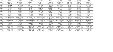
Table 15 The mean and standard deviations of different mutation operators (ADM and L´evy distribution) on different function classes.

Fg ADM1,2,6 ADM10,12,13 ADM16,19,23 α= 1.0 α= 1.2 α= 1.4 α= 1.6 α= 1.8 α= 2.0

F3 _{Std Dev}Mean _(1850.8)4255.7 _(1581.5)3792.5 _(4419.0)9640.8 _(1179.3)2828.6 _(1372.2)3241.0 _(1486.6)2945.1 _(1956.8)3431.5 _(2293.6)3802.6 _(2048.7)4519.7

F4

Mean 38.09 34.55 52.12 31.61 34.66 34.88 38.81 39.12 42.97

Std Dev (9.97) (7.62) (10.86) (7.91) (7.44) (7.84) (8.41) (9.18) (7.12)

F5 _{Std Dev}Mean _(6.63)-6.50 _(5.53)-7.25 _(16.27)5.93 _(6.18)-7.61 _(6.39)-8.19 _(5.30)-6.37 _(6.12)-6.76 _(6.32)-5.37 _(8.11)-3.77

F7 _{Std Dev}Mean 0.0700_(0.02) 0.0584_(0.02) 0.1276_(0.06) 0.0354_(0.01) 0.0401_(0.01) 0.0519_(0.02) 0.0657_(0.03) 0.0723_(0.02) 0.1133_(0.04)

F8

Mean -11205.1 -11318.7 -10484.1 -11111.0 -10503.4 -10089.0 -9664.8 -8949.3 -8072.7

Std Dev (289.4) (358.7) (414.2) (444.4) (479.1) (518.7) (597.4) (589.9) (742.4)

F9 _{Std Dev}Mean -10.2267_(3.16) -10.2257_(3.16) -10.1072_(3.25) -10.2207_(3.16) -10.2238_(3.16) -10.1823_(3.16) -10.0411_(3.11) -9.1189_(3.65) -7.1658_(3.66)

F11 _{Std Dev}Mean 0.0246_(0.12) 0.0039_{(0.01) (18.61)}10.66 0.0011_(0.003) 0.0169_(0.03) 0.0313_(0.07) 0.0402_(0.06) 0.0639_(0.15) 0.1567_(0.30)

F14

Mean 1.0662 0.8955 2.4611 0.7973 0.9778 1.0578 1.1140 1.0665 1.2546

Std Dev (1.17) (0.56) (2.28) (0.38) (0.53) (0.79) (0.70) (0.62) (0.75)

F15 _{Std Dev}Mean 0.0453_(0.02) 0.0415_(0.02) 0.0465_(0.02) 0.0411_(0.02) 0.0426_(0.02) 0.0433_(0.02) 0.0426_(0.02) 0.0464_(0.02) 0.0446_(0.02)

F17 _{Std Dev}Mean 4.942067975_(2.77) 4.942067975_(2.77) 4.942067975_(2.77) 4.942067978_(2.77) 4.942067978_(2.77) 4.942067979_(2.77) 4.942067977_(2.77) 4.942067978_(2.77) 4.942067977_(2.77)

F18

Mean 4.510484905 4.510484905 4.510484889 4.510485582 4.510485593 4.510485625 4.510485455 4.510485479 4.510485176

Std Dev (1.12) (1.12) (1.12) (1.12) (1.12) (1.12) (1.12) (1.12) (1.12)

F20 _{Std Dev}Mean -4.9265_(1.97) -4.8417_(2.06) -4.9847_(1.98) -4.6685_(2.09) -4.6149_(2.11) -4.6951_(2.09) -4.5936_(2.17) -4.8405_(2.04) -4.6868_(2.15)

F21 _{Std Dev}Mean _(7.19E+06)-6.03E+06 _(9.35E+06)-5.29E+06 -5.56E+07_{(7.24E+07) (2.17E+07)}-4.75E+06 _(6.49E+06)-2.89E+06 _(1.99E+07)-6.24E+06 _(4.31E+06)-2.23E+06 _(1.35E+07)-5.84E+06 _(7.83E+06)-4.30E+06

F22

Mean -4.48E+07 -6.60E+06 -7.19E+07 -3.29E+06 -4.46E+06 -3.32E+06 -1.04E+07 -4.06E+06 -4.29E+07

[image:9.612.130.690.251.502.2]