BINK : Biological Binary Keypoint Descriptor

Accepted Manuscript

Title: BINK: Biological Binary Keypoint Descriptor

Author: M´ario Saleiro Kasim Terzi´c J.M.F. Rodrigues J.M.H.

du Buf

PII:

S0303-2647(16)30315-X

DOI:

https://doi.org/doi:10.1016/j.biosystems.2017.10.007

Reference:

BIO 3794

To appear in:

BioSystems

Received date:

25-11-2016

Revised date:

28-9-2017

Accepted date:

11-10-2017

Please cite this article as: M´ario Saleiro, Kasim Terzi´c, J.M.F. Rodrigues, J.M.H. du

Buf, BINK: Biological Binary Keypoint Descriptor,

<![CDATA[BioSystems]]>

(2017),

https://doi.org/10.1016/j.biosystems.2017.10.007

Accepted Manuscript

BINK: Biological Binary Keypoint Descriptor

M´ario Saleiroa_{, Kasim Terzi´c}b_{, J.M.F. Rodrigues}a_{, J.M.H. du Buf}a

a_{Vision Laboratory, LARSyS, FCT&ISE, University of the Algarve, Faro, Portugal} b_{School of Computer Science, University of St. Andrews, Scotland, UK}

Abstract

Learning robust keypoint descriptors has become an active research area in the past decade. Matching local features is not only important for computational applications, but may also play an important role in early biological vision for disparity and motion processing. Although there were already some floating-point descriptors like SIFT and SURF that can yield high matching rates, the need for better and faster descriptors for real-time applications and embedded devices with low computational power led to the development of binary descriptors, which are usually much faster to compute and to match. Most of these descriptors are based on purely computational methods. The few descriptors that take some inspiration from biological systems are still lagging behind in terms of performance. In this paper, we propose a new biologically inspired binary keypoint descriptor: BINK. Built on responses of cortical V1 cells, it significantly outperforms the other biologically inspired descriptors. The new descriptor can be easily integrated with a V1-based keypoint detector that we previously developed for real-time applications.

Keywords: Descriptor, Cortical cells, Keypoints, Applications, Bio-inspired

1. Introduction

During the last decades, the modeling of processes in vi-sion has been attracting more and more attention. Models of simple, complex and end-stopped cells in visual area V1 have been developed and these models have been used for line, edge and keypoint detection (Rodrigues and du Buf, 2006, 2009). Lines and edges have been successfully used for multiple ap-plications like object segregation, scale selection, saliency maps and disparity maps (Rodrigues et al., 2012), optical flow (Far-rajota et al., 2011), face detection and recognition (Rodrigues and du Buf, 2006), facial expression recognition (Sousa et al., 2010), etc. The model for keypoint detection was computation-ally too expensive to be used in real-time applications at the time it was developed, but recent advances in computer hard-ware and code optimizations led to a much faster model that can now be used in real time (Terzic et al., 2015). However, although keypoints indicate the location of specific events in an image, they do not contain information about the regions where they are located: the local image structure. For keypoint matching across images it is necessary to take the local image information around a keypoint and to code this, building a local image descriptor for every single keypoint. These descriptors must be robust to image variations, like changes in illumina-tion, rotaillumina-tion, translaillumina-tion, etc.

Descriptors characterize local image regions by means of a compact numerical representation which should be consistent under a wide range of image transformations. A metric such as Euclidean distance in descriptor space can then provide a measure of similarity between two image patches. Robustness and reliability of modern descriptors have made them indis-pensable in countless applications of Computer Vision, such as image stitching, optical flow and object recognition and

track-ing. Although there are already some very robust and reli-able histogram-based descriptors such as SIFT (Lowe, 2004) and SURF (Bay et al., 2008), which are floating-point descrip-tors that can be used with the Euclidean distance metric, there has been a more recent trend towards binary descriptors such as ORB (Rublee et al., 2011) and BRISK (Leutenegger et al., 2011). These encode a region by a bit vector and typically

use the Hamming distance in the matching process1_{. These}

descriptors have therefore many advantages over the floating-point ones: reduced memory and bandwidth requirements, and faster extraction and matching. This makes them ideal for a growing number of real-time applications and embedded vices with low computational power. Some recent binary de-scriptors have been shown to be on par with histogram-based methods, or even excelled them in some test scenarios (Trzcin-ski et al., 2013).

It is generally accepted that the brain actively constructs explanations for its sensory inputs (Bastos et al., 2012), and several predictive coding models have appeared in the litera-ture (Larkum, 2013; Mumford, 1992; Mumford and Lamme, 1998). There has been much research into hierarchical mod-els and intermediate representations for fast object recognition (Fukushima, 2003; Serre et al., 2007), but feature matching may occur already at the earliest stages of vision, especially in the case of stereo disparity and motion processing. We note that binary descriptors can neatly represent excitation patterns of neural populations, and that their dissimilarity in terms of Ham-ming distance can be easily computed by networks of integrate-and-fire neurons (Vogels and Abbott, 2005). Pairwise

compari-1_{When using a processor with SSE4.2 instructions, matching can be done}

Accepted Manuscript

a comparison between simple and efficient codes built directly

from the responses of V1 cells. This could explain the speed and accuracy of feature matching at the earliest stages of vision. The remaining challenge then is to create a neuronally

plausi-ble method for efficiently extracting binary codes from V1

re-sponses, which can compare in performance to the best descrip-tors in Computer Vision. Some recent binary descripdescrip-tors such as FREAK (Alahi et al., 2012) and BRISK (Leutenegger et al., 2011) were partly motivated by biological vision, but their per-formance is still poor compared to the state of the art in descrip-tor matching (Trzcinski et al., 2013). Our work addresses this problem by learning receptive fields needed to construct good binary codes based on the responses of cortical V1 cells.

Two things are often considered to be important when con-structing a binary descriptor: (i) compact representation, thus reducing storage and bandwidth costs, and (ii) low redundancy between bits, since the Hamming metric implicitly assumes their independence. In this paper, we present a compact bi-nary biological local descriptor built from responses of cortical V1 cells. The coding of the responses is trained on 200K pairs of image patches using LDAHash (Strecha et al., 2012). This allows to create a projection matrix that minimizes the in-class covariance and maximizes the covariance across classes. Each bit of the descriptor is then computed through a linear combi-nation of cell responses. The result of the linear combicombi-nation is thresholded to binarize the output. From a biological point of view, we can consider each bit as a cell that takes input from

multiple V1 cells, each one with a different weight. Depending

on the linear combination of the inputs, the cell may fire (out-put one), or not (zero). The resulting binary vectors can then be matched by using the Hamming distance.

We emphasize that we explore the simplest cell model, namely (1) dendrites at fixed, periodic positions, (2) a

projec-tion matrix which mimicks fixed dendritic transmission coeffi

-cients, (3) linear summation, and (4) the cell response is bina-rized to simulate firing: spike or no spike. As written above, integrate-and-fire neurons can compute the Hamming distance (Vogels and Abbott, 2005). Furthermore, cell summation is ap-plied without any saturation. In artificial neural networks, often nonlinear functions are applied, like a logistic or the rectified linear RELU function. Further research must reveal whether other cell models, for example with nonlinear functions, can yield better results at the expense of more calculations. How-ever, there is some evidence that layer 4C in monkey V1 lin-earizes input from the LGN (Westover and Anderson, 2003).

We will show that our descriptor outperforms all biologically inspired descriptors proposed in the literature, and that it ap-proaches the matching performance of the best binary descrip-tors, even outperforming the SIFT-based LDAHash descriptor. During the development of the proposed descriptor we per-formed extensive tests, trying cell responses with several

com-binations of scales, with different maximum pooling steps and

different pooling sizes. We also experimented with applying the

same approach to biological HMAX and HMIN features instead of V1 cell responses. Since the developed descriptor is compact and takes V1 cell responses as input, it is fast to compute and it

can be used for real-time applications. By integrating the new descriptor with the previously developed V1 keypoint extractor (Terzi´c et al., 2013a; Terzi´c et al., 2013b; Terzic et al., 2015), a biologically motivated keypoint extraction, description and matching pipeline is achieved.

In the next section related work concerning keypoint descrip-tors will be described. Section 3 details the methods that were used to build binary descriptors, and Section 4 deals with the optimization experiments in order to improve the performance. This ends with performance comparisons with other biological and non-biological descriptors and some considerations con-cerning the processing time (Section 5). In the last Section 6 conclusions and suggestions for future work will be presented.

2. Related work

Image regions are often described in terms of gradient his-tograms collected in predefined sampling regions (Bay et al., 2008; Dalal and Triggs, 2005; Lowe, 2004). Although such his-tograms have been considered the absolute state of the art for a long time, they have a large dimensionality. They require a lot of storage capacity and this results in comparably slow match-ing. Subsequent work has reduced dimensionality by using subspace methods (Ke and Sukthankar, 2004) or compression (Chandrasekhar et al., 2009), while keeping most of the bene-fits of the original methods. An appealing alternative approach is based on binary descriptors which can be matched by using the Hamming distance. Early binary descriptors were based on the BRIEF descriptor, which employed pairwise compar-isons of gradients or partial derivatives (Calonder et al., 2012). BRIEF was later modified to take advantage of discriminative projections (Trzcinski and Lepetit, 2012) and keypoint domi-nant orientation (Rublee et al., 2011). Improved sampling pat-terns were shown to boost performance while still using gradi-ents (Alahi et al., 2012; Leutenegger et al., 2011). Descriptors such as BRIGHT (Iwamoto et al., 2013) introduced a variable bit-string length for mobile applications. An alternative, but very popular way to obtain binary descriptors, is by quantiz-ing more complex descriptors (Strecha et al., 2012; Gong et al., 2013a,b).

Recently, focus has shifted towards learning efficient

descrip-tors, which was aided by the availability of large datasets of registered image patches (Brown et al., 2011). Approaches in-clude learning the Mahalanobis distance (Jain et al., 2012), su-pervised hashing (Liu et al., 2012; Wang et al., 2010) and LDA (Strecha et al., 2012; Gong et al., 2013b). Research has also fucused on learning not only feature weights, but also the best pooling strategy (Brown et al., 2011; Simonyan et al., 2014). Most impressive results so far have been achieved by a boost-ing approach (Trzcinski et al., 2013), which jointly optimizes both feature weights and the pooling strategy. Like in our ap-proach, each subsequent bit is optimized to correct the mis-matches which are left after learning the previous bits.

Accepted Manuscript

creating a hierarchy with intermediate features of increasing invariance, such as alternations of pooling and maximum op-erations which simulate stacked layers of simple and complex cells, the HMAX model (Fukushima, 2003; Serre et al., 2007), or intermediate-level convolutional kernels in deep neural net-works (Schmidhuber, 2012). However, these features were op-timized for object classification, not keypoint matching. While BRISK (Leutenegger et al., 2011) and FREAK (Alahi et al., 2012) use biologically-motivated sampling patterns, they make no use of cortical simple and complex cells. Descriptor learn-ing of Brown et al. (2011) comes closest, by uslearn-ing cortically-inspired filters similar to HMAX (Serre et al., 2007). Binary

trees were used for efficient histogram compression by

Chan-drasekhar et al. (2009), but the resulting descriptors require a special matching procedure and they are based on histograms instead of biological features.

The novelty of the present work lies in two aspects: (i) only biologically plausible V1 features will be used, so the descrip-tor can be implemented using a neural architecture; and (ii) to our knowledge, we present the first system that can perform keypoint detection, feature extraction and matching using only biologically plausible features and processes. We note, like Brown et al. (2011), that cortical cells perform many operations which can be used for descriptor coding: they are orientation and scale selective, they pool over spatial regions of varying sizes and shapes, and they respond strongly to discontinuities (gradients). Unlike most descriptor learning approaches, here the goal is not to create a short descriptor; we are more inter-ested in creating a simple coding mechanism that can be used for disparity and optical flow in the earliest stages of vision and that can also be applied in some object recognition applications. In this paper, we show that the coding of V1 features can sum-marize the local image content by relatively short binary codes that allow for robust patch matching, outperforming any other biologically inspired image descriptors and closely approach-ing the non-biologicals but state-of-the-art descriptors.

3. Methods

In order to build and test the descriptors we used two datasets: Notre Dame (the cathedral in Paris, France) and Yosemite (the Natural Park in California, USA) (Brown, 2011). Both sets contain image patches sampled from 3D

reconstruc-tions of interest points, i.e., 64×64 pixels in grayscale, with

variations in viewpoint, distance, contrast and brightness; see

Fig. 1.Matchingpatches are from the same interest points with

a maximum of 5 pixels difference in position, 0.25 octave in

scale andπ/4 radians in angle.Non-matchingpatches have the

same variations but are from different interest points. For

train-ing we used 200K patch pairs from the Notre Dame dataset (100K matches and 100K non-matches) and for evaluation we used 100K patch pairs from the Yosemite dataset (50K matches and 50K non-matches), so that we could compare our results with those obtained by Trzcinski et al. (2013).

All patches were resized to 32×32 pixels in order to speed up

processing, after which responses of even and odd simple cells

Figure 1: Sample patches from the Notre Dame (top two rows) and Yosemite (bottom) datasets that show small differences in terms of scale, displacement, rotation, contrast and brightness.

and of complex cells were computed (see below). Since we ap-plied up to 8 cell orientations and 7 cell scales, in principle it is

possible to compute 3×8×7×322_{features for each patch. The}

total number of 172,032 is excessive for any real-time applica-tion. Therefore, the basic idea is to construct an optimal pro-jection matrix which also reduces the number of features, and

to experiment with different feature selections and sampling or

pooling strategies.

We extracted cell responses from all the image patches of the Notre Dame set at multiple scales and orientations and then applied the LDAHash (Strecha et al., 2012) method to con-struct a projection matrix that minimizes the in-class covariance (matching patch pairs) and maximizes the covariance across classes (the non-matching patch pairs). Then we applied this projection matrix to the cell responses of the training data in order to determine the optimal threshold vector for binarizing each projected feature value. To evaluate the results we used the Yosemite dataset. In the following subsections each step will be described in detail.

3.1. Training and evaluation

The training set serves to determine an optimal projection (rotation) matrix together with an optimal threshold vector which must be applied to all image patches and their features of a real application, like stereo disparity or optical flow. Once such a matrix and vector have been determined by using the training data, exactly the same procedure must be applied to other data of the real application: the same cell selection, fil-ter orientations, scales and pooling scheme. In other words,

the Notre Dame training data are usedonce for constructing

a matrix and corresponding vector, and these are then applied in robot vision, for example. The Yosemite test data are com-pletely irrelevant.

Here, in this paper, the goal is to experiment with diff

er-ent parameter selections: responses of simple and/or complex

cells, the number of cell orientations and their scales, etc. This

Accepted Manuscript

are used to determine one matrix andone vector. Then,

ex-actly the same parameters and matrix plus binarization vector are applied to the Yosemite test data for evaluation purposes: now matching scores are systematically thresholded in order to count true and false positive matches for constructing ROC curves. These curves only serve to gain insight into the

perfor-mance of the different parameter selections. At the end, once

we can draw firm conclusions about which parameter selections are best, one selection must be applied to the training data in or-der to determine a final projection matrix and its corresponding binarization vector.

3.2. V1 cortical cells

In cortical area V1 there are different types of cells: simple,

complex and end-stopped. These cells are thought to play an important role in coding the visual input: they allow to extract multiscale lines and edges (Rodrigues and du Buf, 2009) and

keypoints, which are line/edge vertices or junctions, but also

blobs (Rodrigues and du Buf, 2006).

Responses of even and odd simple cells, which correspond to the real and imaginary part of a Gabor quadrature filter

(Rodrigues and du Buf, 2009), are denoted by RE

s,i(x,y) and

RO

s,i(x,y),i indicating the orientation (we usedNθ = 8). The

scalesis given byλ, the wavelength of the Gabor filters, in

pix-els (we usedλ={4,6,8,12,16,24,32}.) Responses of complex cells are modeled by the modulus

Cs,i(x,y)=[{RE_s,i(x,y)}2+RO_s,i(x,y)2]1/2. (1)

For more details see Rodrigues and du Buf (2006). What is important here is that receptive fields of even and odd simple cells can be seen as derivatives of Gaussians. Hence, like SIFT and derived methods, our method is based on spatial derivatives of the local image structure.

In summary, from each patch we can extract responses of

even and odd simple cells at 8 orientations and 7 different

scales. The responses at each scale are normalized to unit

vec-tor (the L2 norm), and then we perform maximum pooling on

circular receptive fields with a diameter of 4, 6 or 8 pixels and with strides (steps) of 2 or 4 pixels.

3.3. Learning the projection matrix

For learning optimal data projections we apply the LDAHash method (Strecha et al., 2012). As already mentioned, we use two sets of the Notre Dame training data, matching patch pairs and non-matching patch pairs. Let us call these P (positive) pairs in which patches must be matched and N (negative) in

which patches mustnotbe matched. The goal is to obtain a

pro-jection that (a) reduces the number of features, (b) maximizes the probability that P patches are matched, and (c) minimizes the probability that N patches are matched.

Suppose we have one feature (column) vector xof length

n and we want to have a projection y = Px+t whereyhas

dimensionm n,Pis a matrix with dimensionsm×nandt

is a translation vector with dimensionm. The translation vector

serves binarization and will be dealt with later.

The training data contain matching (positive, P) and non-matching (negative, N) patch pairs. Let us call their feature

vectorsxandx0in case of positive, andxandx00in case of

neg-ative pairs. The pairs of feature vectors of positive patches are

“stacked” into two matrices withnfeatures (rows) andN

sam-ples (columns): XandX0_{, here withN =100,000. Likewise,}

for the negative pairs we have two matricesXandX00_.

Now, concerning the LDAHash method, the two matrix pairs

are subtracted: P = X−X0_{andN = X−X}00_{. Then, the two}

covariance matrices ofPandNare computed: ΣPandΣN; and

the ratio matrix after computing the inverse ofΣN:ΣR = ΣPΣ−_N1.

BecauseΣR is positive semidefinite, SVD can be applied for

the eigendecompositionΣR = US UT whereS holds the

(pos-itive) eigenvalues and U the corresponding set of orthogonal

eigenvectors. The orthogonalm×nmatrixPthat minimizes the

trace ofPΣRPTis the projection ofxonto the space spanned by

themeigenvectors with the smallest eigenvalues ofΣR, and

PΣ−_N1/2=S˜_m−1/2U˜TΣ−_N1/2, (2)

where ˜S is them×mmatrix with the smallest eigenvalues and

˜

Uis then×mmatrix with themeigenvectors. We note that the

eigenvectors are divided by the square roots of their

eigenval-ues, and Strecha et al. (2012) keep the normalization byΣ−_N1/2

because this “... makes the projected differencesP(x−x0)

nor-mal and white.”

3.4. Learning the optimal binarization thresholds

To calculate the optimal binarization thresholds we evaluate each dimension independently. We start by finding the

mini-mum, mT, and maximum value, MT, of all projected feature

values in all Notre Dame patches. We created a vector of K

values (we usedK =3000), equidistantly spaced betweenmT

and MT. We then tested all of these values as a binarization

threshold and evaluated which of them provided the largest sum of correct matches and correct non-matches for each individual feature dimension. After evaluating all the dimensions we have

a threshold vector,t, containing as many elements as projected

feature dimensions.

After having the projection matrixPand the optimal

bina-rization threshold vector,t, we can finally compute binary

de-scriptors by thresholding each of the feature dimensions. Each dimension is coded with a 1 if it is bigger than the correspond-ing threshold value, or a 0 if it is smaller.

4. Evaluation

As previously mentioned, for evaluation we used 100K patches of the Yosemite dataset: 50K matching pairs and 50K non-matching pairs, respectively the P(ositive) and N(egative)

sets. This means that the projection matrixPand binarization

vectort, as trained on the Notre Dame dataset for a certain

se-lection of cell responses and pooling step and size, is applied to all patches of the Yosemite set. For each patch pair, the

Ham-ming distanceDHis computed. For example, let us assume that

Accepted Manuscript

con-structing ROC curves in terms of true positives vs. false

posi-tives, we counted the number of true positives in the P set (N_TP)

and the number of false positives in the N set (N_{FP). This was}

done for all numbers of bits. For example, in the case of 10

bits, all pairs withDH≤10 in the P set contributed toN_{TP, and}

all pairs with DH ≤10 in the N set contributed toN_{FP. After}

dividing the two counts by 50K, we have one point of the ROC curve. This procedure yields ROC curves with, in this example, 128 points, of which only the points with a true positive rate between 0.5 and 1, and a false positive rate between 0 and 0.5, are plotted.

We ran multiple tests in the attempt of finding the best

selec-tion of input data: we experimented with different cell scales

λ = {4,6,8,12,16,24,32}, different pooling steps p = {2,4},

and different pooling sizess = {4,6,8}. All patches were

re-sized to 32 ×32 pixels before feature extraction to speed up

evaluation. Pooling means response selection by searching for the maximum response in circular windows with a diameter of e.g. 4 pixels (the pooling size) and this window is shifted e.g. 2

pixels in xand iny(the pooling step). Each scale is evaluated

independently in order to determine the scale’s optimal pooling step and pooling size.

4.1. Cell selection: even simple, odd simple or complex?

The first test was about which cells and combinations of cells contained the most discriminative information: even simple cells, odd simple cells and complex cells. Throughout all our tests we verified that, in most cases, complex cells provided the least discriminative information: since they are computed from combinations of simple cell responses, there is loss of discrim-inative information. On the other hand, even and odd simple cells performed better at most scales, and very similarly. At the

finest scale (λ=4) best results are obtained when using

com-binations of even and odd simple cell responses (95% error rate of 50.2%, as in (Trzcinski et al., 2013): this means that at a true positive rate of 95%, the false positive rate is 50.2%). This re-sult is followed by using only even or only odd cell responses. At all other scales, best results were obtained by using a com-bination of even, odd and complex cells. Worst results at each scale were obtained by using only complex cells.

By combining even and odd simple cell responses, the use of more features leads to the best performance. When com-bining all cell responses there is also an improvement, except

for scale λ = 4. At coarser scales (λ = {8,12,16,24}), the

combination of even, odd and complex cell responses yields the best performance. Since the number of features per cell type becomes smaller, which is due to the subsampling of the image and shrinking of the patch size at coarser scales, com-bining multiple cell types leads to better results. However, in

most cases the difference between combining only even and odd

simple cells and also using complex cells is not very significant, which means that complex cells do not add much more discrim-inative information. The increase in performance by combining simple cell responses with complex cell responses gets smaller

at coarser scales. At scaleλ=32 the result of using even, odd

0 0.05 0.1 0.15 0.2 0.25 0.3 0.35 0.4 0.45 0.5 0.5

0.55 0.6 0.65 0.7 0.75 0.8 0.85 0.9 0.95 1

True

Positive

Rate

False Positive Rate Train: Notre Dame; Test: Yosemite

even,λ=4, s = 6, 128b, 1568 features complex,λ=4, s = 6, 128b, 1568 features odd,λ=4, s = 6, 128b, 1568 features even+odd,λ=4, s = 6, 128b, 3136 features complex+even+odd,λ_{=4, s = 6, 128b, 4704 features}

even,λ=12, s = 4, 128b, 392 features complex,λ=12, s = 4, 128b, 392 features odd,λ=12, s = 4, 128b, 392 features even+odd,λ=12, s = 4, 128b, 784 features complex+even+odd,λ=12, s = 4, 128b, 1176 features even,λ=24, s = 4, 64b, 72 features

complex,λ=24, s = 4, 64b, 72 features odd,λ=24, s = 4, 64b, 72 features even+odd,λ=24, s = 4, 128b, 144 features complex+even+odd,λ=24, s = 4, 128b, 216 features

Figure 2: Comparison of results using different types of cells. In most cases even or odd simple cell responses result in better performance than when using responses of complex cells. Results obtained with even and odd simple cells are very similar. Combining different cell responses may or may not result in better performance, depending on the scale and the cells used. All the plots were generated using a pooling stepp=2 pixels. At scaleλ=24 only 64 bits were used for each individual type of response because the number of features was insufficient to generate a 128-bit descriptor.

and complex cells is worse than when using only even and odd simple cells.

In most cases, best results were obtained by using even and

odd simple cells. To illustrate the differences in performance,

Fig. 2 shows results obtained with 128-bit descriptors built from

features at three different scales, λ = {4,12,24}, and with a

pooling step of 2 pixels. It can be seen that for the three scales shown in Fig. 2 complex cells have a poorer performance than

even or odd simple cells at the same scale. Similar differences

in performance were obtained when testing other scales.

4.2. Scale comparison

As previously mentioned, we tested seven different cell

Accepted Manuscript

0 0.05 0.1 0.15 0.2 0.25 0.3 0.35 0.4 0.45 0.5 0.5

0.55 0.6 0.65 0.7 0.75 0.8 0.85 0.9 0.95 1

True Positive Rate

False Positive Rate Train: Notre Dame; Test: Yosemite

even+odd, λ=4, s = 4, 128b, 3600 features even, λ=6, s = 4, 128b, 1800 features complex+even+odd, λ=8, s = 4, 128b, 1176 features complex+even+odd, λ=12, s = 4, 128b, 1176 features complex+even+odd,λ=16, s = 4, 128b, 216 features complex+even+odd, λ=24, s = 4, 128b, 216 features even+odd, λ=32, s = 4, 16b, 16 features

Figure 3: Comparison of the best results at each of the scales tested. The best result is obtained usingλ = 4 (95% error rate of 49.1%), closely followed byλ =6. As the scale gets coarser, the number of features is reduced and performance also decreases. In all cases we usedp=4.

comparing scales with similar numbers of features (e.g. λ=4

andλ = 6), the finer scales perform slightly better. Figure 3

shows the best results obtained at each of the scales, and it also mentions the number of features used for each of the results.

In addition, Fig. 3 shows that scaleλ=4 yields the best result

when combining responses of even and odd simple cells,

fol-lowed by scaleλ = 6, using only even simple cell responses.

4.3. Pooling region size

The size of the pooling region also influences the perfor-mance of the descriptor. By using a larger pooling region we get fewer features, because of the influence of the patch border

(32×32 pixels), but the features may be more robust and have

a higher invariance to small transformations.

The pooling schemes tested here implement a periodic and continuous sampling pattern. In earlier tests we explored the possibility of extracting structural keypoint information, like

the junction type (L or T or+), and edge orientations and

am-plitudes. In general, the results were not very good because, by definition, responses of simple and complex cells at and around

junctions are influenced by interference effects (du Buf, 1993).

Therefore we apply regular sampling patterns, because they can

capture responses with interference effects and the information

between e.g. edges is also important.

We tested all the scales with pooling regions with diameters of 4, 6 and 8 pixels to determine which pooling size leads to a better performance. Some results are shown in Fig. 4.

From this figure it can be seen that for the three scales a

pool-ing size of s = 4 provides the best results (95% error rate of

48.5%). As the pooling size increases, the number of features

0 0.05 0.1 0.15 0.2 0.25 0.3 0.35 0.4 0.45 0.5

0.5 0.55 0.6 0.65 0.7 0.75 0.8 0.85 0.9 0.95 1

True Positive Rate

False Positive Rate Train: Notre Dame; Test: Yosemite

λ=4, s = 4, 1800 features λ=4, s = 6, 1568 features λ=6, s = 4, 1800 features λ=6, s = 6, 1568 features λ=8, s = 4, 392 features λ=8, s = 6, 288 features

Figure 4: Evaluation of performance for pooling regions with different sizes. At all scales a pooling size of 4 pixels leads to the best results. Performance de-creases with increasing pooling size. Results shown are for 128-bit descriptors built from even simple cell responses with a pooling step of 2 pixels. Results are similar for other cells.

decreases, as does performance. Results for a pooling size of 8 pixels are not shown in the figure, but they were worse than those with sizes of 4 and 6 pixels.

At scaleλ=8 we can see that the performance clearly drops

as the pooling size increases. The same happens at other coarse scales. A bigger pooling size drastically reduces the number of features at coarser scales.

4.4. Pooling step selection

As shown in the previous sections, although a larger number of features usually leads to better results, this is not always true. We therefore tested the influence of increasing the pooling step to evaluate if by cutting down the number of features, especially at finer scales, we could obtain a similar performance. This could be useful to improve the descriptor computation speed.

The pooling step was increased to 4 pixels, which effectively

reduces the number of features to 1/4 of the features extracted

with a pooling step of 2 pixels. Some results are shown in Fig. 5. It can be seen that by reducing the number of features

to 1/4 of the total number of features, the performance

signif-icantly decreases. This means that most of the features con-tain useful discriminative information and cannot be discarded

without affecting performance.

4.5. Dimensionality of the descriptor

In this step we tested the influence of the dimensionality, or

number of bits,nbits, on the performance of the descriptor. We

evaluated the best results from the two scales with best results

(λ=4 andλ=6 with a pooling size of 4 pixels and a pooling

Accepted Manuscript

0 0.05 0.1 0.15 0.2 0.25 0.3 0.35 0.4 0.45 0.5

0.5 0.55 0.6 0.65 0.7 0.75 0.8 0.85 0.9 0.95 1

True Positive Rate

False Positive Rate Train: Notre Dame; Test: Yosemite

λ=4, s = 4, p = 2, 1800 features

λ=4, s = 4, p = 4, 450 features λ=6, s = 4, p = 2, 1800 features λ=6, s = 4, p = 4, 450 features

Figure 5: Evaluation of performance of 128-bit descriptors generated from even simple cell responses with pooling steps of 2 and 4 pixels and a pooling size of 4 pixels. There is a clear decrease in performance forp=4.

0 0.05 0.1 0.15 0.2 0.25 0.3 0.35 0.4 0.45 0.5

0.5 0.55 0.6 0.65 0.7 0.75 0.8 0.85 0.9 0.95 1

True Positive Rate

False Positive Rate Train: Notre Dame; Test: Yosemite

λ=4, s = 4, 64 bits λ=4, 128 bits λ=4, 256 bits λ=4, 512 bits λ=6, s = 4, 64 bits λ=6, 128 bits λ=6, 256 bits λ=6, 512 bits

Figure 6: Comparison of results using 4 different numbers of bits at scalesλ=4 (blue) andλ=6 (red). Best results at both scales are obtained using 128 bits, but for scaleλ=6 results with 256 bits are very similar.

Figure 6 shows that the performance peaks at 128 bits and it decreases as the number of bits increases. Using 256 bits re-sults in a drop in performance and a bigger drop occurs when using 512 bits. Results using 64 bits are worse than those with 256 bits for small false positive (FP) rates, but they are better at larger FP rates. These results are consistent with the dimension-ality evaluation done for LDAHash; see Fig. 6 from Trzcinski et al. (2013).

0 0.05 0.1 0.15 0.2 0.25 0.3 0.35 0.4 0.45 0.5

0.5 0.55 0.6 0.65 0.7 0.75 0.8 0.85 0.9 0.95 1

True Positive Rate

False Positive Rate Train: Notre Dame; Test: Yosemite

even, λ=4, s = 4 even+odd, λ=4, s = 4 complex, all scales

all best single scale results combined

Figure 7: Comparison between the best 128-bit single-scale result previously obtained (λ =4 with a pooling size of 4 pixels and a pooling step of 2 pix-els) and three 128-bit descriptors built from different combinations of cell re-sponses. Only the combination of complex cells at all scales performed worse than the best single scale result.

4.6. Combining different scales

Up to this point we evaluated the influence of different

pa-rameters on descriptor performance for each scale individu-ally. However, in cortical area V1 cell responses at multiple scales are combined to create higher level representations. Tak-ing this into account, it can perhaps be expected that by com-bining cell responses at several scales a better result may be achieved. Therefore we experimented with a few combinations of responses at all scales. We also tested what happens when we combine the cells that provided the best result at each individual scale. Figure 7 illustrates the results obtained.

From Fig. 7 it can be seen that two of the three different cell

combinations perform much better than the best single-scale, even simple cell 128-bit descriptor: (1) the combination of even

and odd simple cells at scaleλ=4; and (2) the combination of

all best single-scale results. It can also be seen that the descrip-tor built only from even simple cells provides a better result than that built only from complex cells at all scales. The best result is obtained with the combination of all the best single-scale results (95% error rate of 35.1%) but it is very similar to the one obtained by combining even and odd simple cells at

scaleλ=4 (95% error rate of 35.8%). From the plot it seems

once more that responses of complex cells are less discrimina-tive than those of even or odd simple cells.

4.7. Testing HMAX features

Accepted Manuscript

0.5 0.55 0.6 0.65 0.7 0.75 0.8 0.85 0.9 0.95 1

True Positive Rate

False Positive Rate Train: Notre Dame; Test: Yosemite

even, λ=4, s = 4, 128 bits even+odd, , s = 4, 128 bits HMAX, 128 bits

HMAX + even, λ=4, s = 4, 128 bits all scales

Figure 8: HMAX features are much weaker than our even simple cell responses at scaleλ=4, even considering that we could use 8150 HMAX features and only 1800 even simple cell features. When combining them with our even simple cell responses, the performance becomes slightly better but it is still worse than the result when using only even simple cell responses.

even simple cell responses at scaleλ = 4. The results can be

seen in Fig. 8. Using only HMAX features results in a poor performance. Using HMAX features together with even sim-ple cell responses leads to a result which is only slightly better. Relative to the best result that we had up to this point (all even and odd simple cells at all scales with a pooling step of 2 pix-els), we can see that performance is much worse. Even using

only even simple cell responses at scale λ = 4 yields a better

result. Apart from the lower performance, HMAX features also have the disadvantage of taking much more time to compute than our simple cell responses. This makes them unsuitable for any real-time applications with the computational power which is currently available.

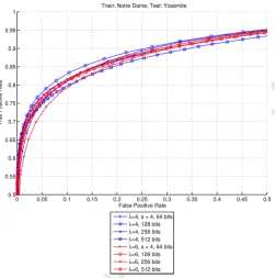
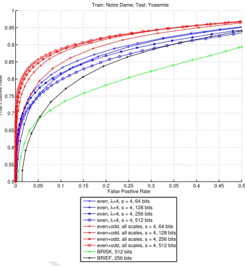
4.8. Comparison with other biologically inspired descriptors In this section we compare the descriptor that we developed and the biologically inspired descriptors BRISK (512 bits) and BRIEF (256 bits). Figure 9 shows that the descriptor that we developed significantly outperforms both of them. The 64-bit

version of our descriptor, either using only scaleλ=4 or using

the combination of even and odd simple cells at all tested scales,

is already good enough to clearly outperform them. They

have respectively false positive rates of 48.5% (single-scale)

and 35.8% (multi-scale) for a 95% error rate, versus 55.0% of

BRIEF and 73.2% of BRISK, which use 4 and 8 times more

bits. If we consider a direct comparison in terms of bits, the

256 bit version of our descriptor at scaleλ=4 has a 95% error

rate of 54.3%, which is only 0.7% better than BRIEF, but it is

much better at low false positive rates. Comparing the present

descriptor built from multiple scales, the 95% error rate diff

er-ence to BRIEF is bigger: 19.8%. Making the same comparison

with BRISK, we have 95% error rate differences of 37.7% and

0 0.05 0.1 0.15 0.2 0.25 0.3 0.35 0.4 0.45 0.5

0.5 0.55 0.6 0.65 0.7 0.75 0.8 0.85 0.9 0.95 1

True Positive Rate

False Positive Rate Train: Notre Dame; Test: Yosemite

even, λ=4, s = 4, 64 bits even, λ=4, s = 4, 128 bits even, λ=4, s = 4, 256 bits even, λ=4, s = 4, 512 bits even+odd, all scales, s = 4, 64 bits even+odd, all scales, s = 4, 128 bits even+odd, all scales, s = 4, 256 bits even+odd, all scales, s = 4, 512 bits BRISK, 512 bits

BRIEF, 256 bits

Figure 9: Comparison of our descriptor performances with other biologically inspired descriptors BRIEF and BRISK. Our descriptor, either using only even simple cells at scaleλ=4 or using a combination of even and odd simple cells at multiple scales, outperforms both BRIEF and BRISK, even when using four or eight times less bits.

14.8%. The present descriptor clearly outperforms the other

bi-ologically inspired descriptors BRIEF and BRISK, even when using four or eight times less bits.

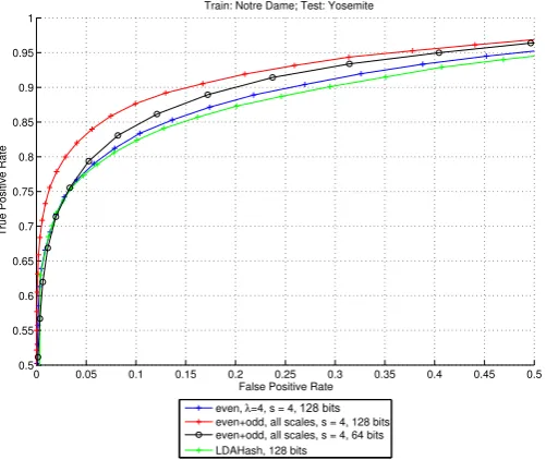
4.9. Comparison with the SIFT-based LDAHash descriptor

Figure 10 shows that both our single-scale and multi-scale 128-bit descriptors outperform the SIFT-based 128-bit tor LDAHash, a state-of-the-art, but non-biological descrip-tor. The present descriptors have 95% error rates of 48.5% (single-scale) and 35.8% (multi-scale), which are both better than LDAHash (52.9%). When considering low false positive rates, our descriptors are still better than LDAHash, and even when using a 64-bit version of the multi-scale descriptor we still get better results (a 95% error rate of 40%).

4.10. Computation time

After showing that the new descriptor outperforms the other biologically-inspired descriptors BRIEF and BRISK and also the non-biological, SIFT-based descriptor LDAHash, comes the question: can it be used as alternative to other descriptors cur-rently used in real-time applications? To evaluate the computa-tion time in a proper way the processing time was split into two steps: feature extraction and descriptor computation.

We measured the average time of feature extraction over

1000 patches of 32×32 pixels, thus implicitly assuming one

keypoint at the center of each patch. For the single scale

fea-tures (λ =4) the average time was 2.15 ms and for the

Accepted Manuscript

0 0.05 0.1 0.15 0.2 0.25 0.3 0.35 0.4 0.45 0.5

0.5 0.55 0.6 0.65 0.7 0.75 0.8 0.85 0.9 0.95 1

True Positive Rate

False Positive Rate Train: Notre Dame; Test: Yosemite

even, λ=4, s = 4,

even+odd, all scales, s = 4, 128 bits

LDAHash, 128 bits

even+odd, all scales, s = 4, 64 bits

128 bits

Figure 10: Comparison of our descriptors with the non-biologically inspired descriptor LDAHash.

2.35 ms. Times were measured on a computer with a quad-core

processor running at 2.4 GHz and with OpenMP for parallel

processing. Regarding theconstructionof the descriptor, it is

a much faster process and takes only an average time of 0.45

ms for only scale λ = 4 and 0.52 ms for the combination of

several scales. However, in this step no parallel processing was applied and there is still room for optimization. Since feature extraction and descriptor computation take a few milliseconds, processing times are good enough for some real-time applica-tions. However, the processing time can be greatly reduced by using a more modern processor. Another option is to use our GPU implementation of feature extraction and keypoint detec-tion (Terzic et al., 2015). This can reduce computadetec-tion time very significantly, while leaving the CPU processor free for other processes.

5. Applications

In this section some applications will be shown of the de-scriptor that we developed. As referred to in previous sections, descriptors can be used for early vision processes, such as opti-cal flow and stereo vision, but also for object recognition.

5.1. Optical flow

Optical flow is the motion pattern caused by moving objects in a visual scene. It can be described by the motion or displace-ment vectors of entire objects or parts of them between suc-cessive time frames. From a biological point-of-view, there are strong arguments indicating that neurons in a specialized region of the cerebral cortex play a very important role in flow anal-ysis (Wurtz, 1998). According to William and Charles (2008), neuronal responses to flow are shaped by visual strategies for steering, and according to Warren and Rushton (2009), the flow processing has a very important role in the detection and esti-mation of scene-relative object movement during egomotion.

Using our previously developed keypoint detector (Terzic et al., 2015), we extracted keypoints in successive camera frames. Then we applied our new descriptor to match keypoints from one frame to the other, thus obtaining each keypoint’s dis-placement vector. Since keypoint disdis-placement is expected to be relatively small from one frame to the next one, depend-ing on frame rate, we can limit keypoint matchdepend-ing to a specific range, and not waste computation time in matching very distant keypoints. Since our descriptors are binary and we only have to match each descriptor against a few other descriptors, optical

flow can be determined in a very simple, fast and effective way.

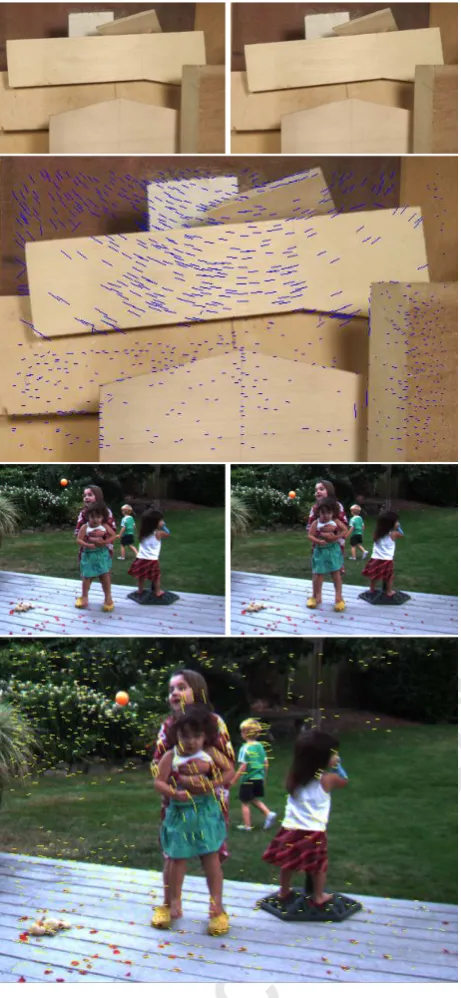
Figure 11 shows two examples of optical flow estimated by using our cortical keypoint detector and descriptor. Keypoints

were extracted at scale λ = 4 and annotated by the 128-bit

single-scale descriptor, also using onlyλ = 4. The matching

was done between each keypoint in the first frame and all key-points within a 30 pixel distance in the second frame. The top

video in Fig. 11 has a resolution of 584×388 pixels and an

av-erage of 1932 keypoints per frame. The bottom video has a size

of 640×480 pixels with an average of 1594 keypoints.

5.2. Stereo vision

Stereo vision is another important process in our brain. It al-lows us to estimate distances to obstacles and objects and is es-pecially important for navigation. In our primary visual cortex we have binocular neurons which take input from both left and right eyes and integrate the signals together to create a percep-tion of depth. These cells are selective, usually tuned to specific disparity ranges. We assume that each binocular neuron takes as input higher level representations from points on the same epipolar line from left and right images, compares them, and fires if the representations are similar. These higher level repre-sentations could be our keypoints and their descriptors.

Looking at the problem from a computational point of view, we can compute disparity maps through the following process: instead of applying keypoint detection we can code each pixel from the left and right images by using our keypoint descriptor.

Then we match each coded pixel of the left image to the nextK

pixels on the same epipolar line of the right image. The hori-zontal displacement between the two best-matching pixels then corresponds to the disparity value of that pixel.

Figure 12 shows an example of a disparity map, withK=30.

Since the goal of this section is only to show the possibility of applying the descriptors for stereo matching, no extra pre-or post-processing was applied. If the goal was to achieve a state-of-the-art stereo algorithm, further processing is neces-sary (Martins et al., 2015). However, rough stereo maps are

sufficient for robot navigation and obstacle avoidance.

5.3. Object recognition

Accepted Manuscript

key-point descriptors. Rows 1 and 3 show two successive frames from two different sets. Rows 2 and 4 show the optical flow results obtained from matching key-points between the two frames. The images belong to the Middlebury Optical Flow dataset (Scharstein, 2009a)

.

the ones of the labeled templates. Once we have at least 30% of matching keypoints between the query image and a template, we can assume that a match has been detected. Figure 13 shows an example of matching a cup. We are able to perform ob-ject recognition in real time and by using several scales we can

match objects that have different sizes. In the case of Fig. 13,

we applied scalesλ =8 and 16 for single-scale descriptors of

128 bits.

Figure 12: Example of stereo matching using our descriptor to match pixels from the left image to the right image. The image is part of the Middlebury dataset for stereo vision (Scharstein, 2009b).

Figure 13: Example of object recognition using our keypoint descriptors, ex-tracted at scalesλ=8 andλ=16. Since the cup in the left image is at a smaller scale than the one in the right image, the descriptors from scaleλ=8 in the left image correctly match those from scaleλ=16 in the right image.

6. Conclusions

Accepted Manuscript

cell responses at multiple scales. According to the experiments it was verified that by using more scales and more even and odd simple cell responses, the result is usually better. Complex cells, on the other hand, do not add much useful information. Overall, best results were obtained with descriptors of 128 bits. As further work we intend to create a GPU implementation of the descriptor construction process which can be integrated with the keypoint detection implementation. Since keypoint de-tection is also based on responses of simple and complex cells, the responses of these cells are readily available for the descrip-tor process. The result will be a complete keypoint detection and description framework that is fast enough for several real-time applications, such as real-real-time vision for biologically in-spired robotics. Another step for the future is to repeat the work described in this paper for building descriptors with a smaller number of features and with a smaller number of bits. Although these descriptors will perform worse than the ones tested in this paper, they may still be useful to speed up processes such as optical flow and stereo vision, which, as shown, can be imple-mented by matching descriptors against a small set of other

de-scriptors. Our brain performs these processes very efficiently

and concurrently.

Acknowledgements

This work was supported by the EU under the FP-7 Grant ICT-2009.2.1-270247 NeuralDynamics, the Portuguese Foundation for Science and Technology (FCT), LARSyS

[UID/EEA/50009/2013] and by FCT PhD grant to the 1st

au-thor SFRH/BD/71831/2010.

References

Alahi, A., Ortiz, R., Vandergheynst, P., 2012. FREAK: Fast retina keypoint. Proc. Int. Conf. Computer Vision and Pattern Recognition (CVPR), 510– 517.

Bastos, A. M., Usrey, W. M., Adams, R. A., Mangun, G. R., Fries, P., Friston, K. J., 2012. Canonical microcircuits for predictive coding. Neuron 76 (4), 695–711.

Bay, H., Tuytelaars, T., van Gool, L., 2008. SURF: Speeded-up robust features. Computer Vision and Image Understanding 110 (3), 346–359.

Brown, M., 2011. Learning local image descriptors data. Online; accessed 17-Feb-2015.

URLhttp://www.cs.ubc.ca/ mbrown/patchdata/patchdata.html

Brown, M., Hua, G., Winder, S., 2011. Discriminative learning of local im-age descriptors. IEEE Trans. on Pattern Analysis and Machine Intelligence 33 (1), 43–57.

Calonder, M., Lepetit, V., ¨Ozuysal, M., Trzcinski, T., Strecha, C., Fua, P., 2012. BRIEF: Computing a local binary descriptor very fast. IEEE Trans. on Pat-tern Analysis and Machine Intelligence 34 (7), 1281–1298.

Chandrasekhar, V., Takacs, G., Chen, D., Tsai, S., Grzeszczuk, R., Girod, B., 2009. CHoG: Compressed histogram of gradients a low bit-rate feature de-scriptor. Proc. Int. Conf. Computer Vision and Pattern Recognition (CVPR), 2504–2511.

Dalal, N., Triggs, B., 2005. Histograms of oriented gradients for human de-tection. Proc. Int. Conf. Computer Vision and Pattern Recognition (CVPR), 886–893.

du Buf, J., 1993. Responses of simple cells: events, interferences, and ambigu-ities. Biol. Cybern. 68, 321–333.

Farrajota, M., Rodrigues, J. M. F., du Buf, J. M. H., 2011. Optical flow by multi-scale annotated keypoints: a biological approach. Proc. Int. Conf. on Bio-inspired Systems and Signal Processing (BIOSIGNALS), 307–315.

Fukushima, K., 2003. Neocognitron for handwritten digit recognition. Neuro-computing 51, 161–180.

Gong, Y., Kumar, S., Rowley, H. A., Lazebnik, S., 2013a. Learning binary codes for high-dimensional data using bilinear projections. Proc. Int. Conf. Computer Vision and Pattern Recognition (CVPR), 484–491.

Gong, Y., Lazebnik, S., Gordo, A., Perronnin, F., 2013b. Iterative quantization: A procrustean approach to learning binary codes for large-scale image re-trieval. IEEE Trans. on Pattern Analysis and Machine Intelligence 35 (12), 2916–2929.

Iwamoto, K., Mase, R., Nomura, T., 2013. Bright: A scalable and compcact binary descriptor for low-latency and high-accuracy object identification. Int. Conf on Image Processing, 2915–2919.

Jain, P., Kulis, B., Davis, J. V., Dhillon, I. S., 2012. Metric and kernel learning using a linear transformation. J. of Machine Learning Research 13, 519–547. Ke, Y., Sukthankar, R., 2004. PCA-SIFT: a more distinctive representation for local image descriptors. Proc. Int. Conf. Computer Vision and Pattern Recognition (CVPR), 506–513.

Larkum, M., 2013. A cellular mechanism for cortical associations: an organiz-ing principle for the cerebral cortex. Trends in Neurosciences 36 (3), 141– 151.

Leutenegger, S., Chli, M., Siegwart, R. Y., 2011. BRISK: Binary robust in-variant scalable keypoints. Proc. Int. Conf. Computer Vision (ICCV), 2548– 2555.

Liu, W., Wang, J., Ji, R., Jiang, Y. G., Chang, S. F., 2012. Supervised hash-ing with kernels. Proc. Int. Conf. Computer Vision and Pattern Recognition (CVPR), 2074–2081.

Lowe, D. G., 2004. Distinctive image features from scale-invariant keypoints. Int. J. of Computer Vision 60, 91–110.

Martins, J. A., Rodrigues, J. M., du Buf, H., 2015. Luminance, colour, viewpoint and border enhanced disparity energy model. PloS one 10 (6), e0129908.

Mumford, D., 1992. On the computational architecture of the neocortex. Biol. Cybern. 66 (3), 241–251.

Mumford, D., Lamme, V. A. F., 1998. The role of primary visual cortex in higher level vision. Vision Research 38 (15-16), 2429–2454.

Mutch, J., 2011. HMIN: A minimal HMAX implementation. Online; accessed 14-Jul-2015.

URLhttp://cbcl.mit.edu/jmutch/hmin/

Rodrigues, J., du Buf, J. M. H., 2006. Multi-scale keypoints in V1 and be-yond: object segregation, scale selection, saliency maps and face detection. BioSystems 2, 75–90.

Rodrigues, J., du Buf, J. M. H., 2009. Multi-scale lines and edges in V1 and be-yond: brightness, object categorization and recognition, and consciousness. BioSystems 95, 206–226.

Rodrigues, J. M. F., Martins, J. A., Lam, R., du Buf, J. M. H., 2012. Cortical multiscale line-edge disparity model. In: Campilho, A., Kamel, M. (Eds.), Image Analysis and Recognition. Vol. 7324 of LNCS. pp. 296–303. Rublee, E., Rabaud, V., Konolige, K., Bradski, G. R., 2011. Orb: An efficient

al-ternative to SIFT or SURF. Proc. Int. Conf. Computer Vision (ICCV), 2564– 2571.

Scharstein, D., 2009a. Middlebury datasets for optical flow. Online; accessed 15-Sept-2015.

URLhttp://vision.middlebury.edu/flow/data/

Scharstein, D., 2009b. Middlebury datasets for stereo vision. Online; accessed 15-Sept-2015.

URLhttp://vision.middlebury.edu/stereo/

Schmidhuber, J., 2012. Multi-column deep neural networks for image classifi-cation. Proc. Int. Conf. Computer Vision and Pattern Recognition (CVPR), 3642–3649.

Serre, T., Wolf, L., Bileschi, S., Riesenhuber, M., Poggio, T., 2007. Object recognition with cortex-like mechanisms. IEEE Trans. on Pattern Analysis and Machine Intelligence 29 (3), 411–426.

Simonyan, K., Vedaldi, A., Zisserman, A., 2014. Learning local feature de-scriptors using convex optimisation. IEEE Trans. on Pattern Analysis and Machine Intelligence, 1573–1585.

Sousa, R., Rodrigues, J. M. F., du Buf, J. M. H., 2010. Recognition of facial expressions by cortical multi-scale line and edge coding. Proc. Int. Conf. on Image Analysis and Recognition (ICIAR) 1, 415–424.

Accepted Manuscript

M. F., Lam, R., du Buf, J. M. H., 2013a. Biological models for active vision: Towards a unified architecture. Proc. Int. Conf. on Computer Vision Systems 7963, 113–122.

Terzi´c, K., Rodrigues, J. M., du Buf, J. H., 2013b. Fast cortical keypoints for real-time object recognition. In: 2013 IEEE International Conference on Image Processing. IEEE, pp. 3372–3376.

Terzic, K., Rodrigues, J. M. F., du Buf, J. M. H., 2015. BIMP: A real-time biological model of multi-scale keypoint detection in V1. Neurocomputing 150, 227–237.

Trzcinski, T., Christoudias, C. M., Fua, P., Lepetit, V., 2013. Boosting binary keypoint descriptors. Proc. Int. Conf. Computer Vision and Pattern Recog-nition (CVPR), 2874–2881.

Trzcinski, T., Lepetit, V., 2012. Efficient discriminative projections for compact binary descriptors. Proc. European Conf. on Computer Vision, 228–242. Vogels, T. P., Abbott, L. F., 2005. Signal propagation and logic gating in

net-works of integrate-and-fire neurons. J. of Neuroscience 25 (46), 10786– 10795.

Wang, J., Kumar, S., Chang, S. F., 2010. Sequential projection learning for hashing with compact codes. Proc. Int. Conf. Machine Learning, 1127– 1134.

Warren, P., Rushton, S., 2009. Optic flow processing for the assessment of ob-ject movement during ego movement. Current Biology 19 (19), 1555–1560. Westover, M. B., Anderson, C. H., 2003. Layer 4c in monkey v1 may linearize

the output of the lgn. Neurocomputing 52, 671–676.

William, K., Charles, J., 2008. Cortical neuronal responses to optic flow are shaped by visual strategies for steering. Cerebral Cortex 18 (4), 727–739. Wurtz, R., 1998. Optic flow: A brain region devoted to optic flow analysis?