Abstract—Segmentation and analysis of histological images provides a valuable tool to gain insight into the biology and function of microglial cells in health and disease. Common image segmentation methods are not suitable for inhomogeneous histology image analysis and accurate classification of microglial activation states has remained a challenge. In this paper, we introduce an automated image analysis framework capable of efficiently segmenting microglial cells from histology images and analysing their morphology. The framework makes use of vari-ational methods and the fast-split Bregman algorithm for image denoising and segmentation, and of multifractal analysis for feature extraction to classify microglia by their activation states. Experiments show that the proposed framework is accurate and scalable to large datasets and provides a useful tool for the study of microglial biology.
Index Terms—microglia analysis, Mumford-Shah, fast split Bregman, fast Fourier transform, multifractal analysis, histology data analysis.
I. INTRODUCTION
M
ICROGLIA are immune cells exclusive to the central nervous system (CNS) and about 1.5 trillion of them reside in the brain and spinal cord [1], [2]. In response to a variety of signals, microglia show a range of phenotypes, from protective to detrimental associated with motility and morphological changes [3]. In the healthy brain, microglia constantly survey the surrounding tissue with extended pro-cesses, clear debris from dead cells, and prune and maintain brain synapses. They are also essential to learning and memory [4], [5], protect neurons from damage, and mediate pain [6], [7]. In response to an injury or infection, microglia initiate an early, protective response by moving towards the site of injury, where they release a cascade of chemicals leading to repair of the damaged area. Microglial activation is a hallmark of chronic neuroinflammation, which is believed to play an important role in a range of brain disorders, which has yet to be fully understood, including stroke, multiple sclerosis, Parkinson’s, Huntington’s and Alzheimer’s disease [8], [9], [10], and can also reflect a neuroprotective behaviour in these chronic conditions [3].The heterogeneity of microglial functions is in part linked to their shape and activation state, and much information can be obtained from their morphological characteristics [11]. Microglial cell shape evolves from a resting fully ramified shape with extending processes and smaller soma, to the
Email –[email protected]
fully activated amoeboid shape with a larger soma and shorter processes [12], [13]. To date, microglia activation has been linked to three distinct functions: a classical pro-inflammatory activation state, an alternative activated anti-inflammatory state and a complementary deactivation state associated with an anti-inflammatory and functional repair phenotype [3]. Classifying microglia activation states in histological images can help pathologists with disease diagnosis [14], provides key information for understanding diseases of the central nervous system [15] and is essential for the validation of in vivo biomarkers that allow the stratification and monitoring of patients and populations at risk [16], [17].
One of the major challenges in quantitative microglial analysis from immunohistological images is the development of automated microglial segmentation methods. Manual or semi-automated segmentation methods are time consuming and require user intervention [18], [19] with an element of subjectivity and inter-observer variability. Image analysis approaches commonly used for quantifying histology that rely on thresholding struggle with inhomogeneous immun-ohistochemistry images, where even staining over a single brain slice can be challenging. Another key challenge is the classification of distinct morphological states from resting-ramified to activated amoeboid, particularly the intermediate states, which is intimately linked to the multiple phenotypes of microglia [11]. Recent work has considered microglia as monofractals, and used a single fractal dimension value to describe the entire microglial structure [20], [11]. However, fractal dimension alone is not enough to discriminate microglia activation states as it only measures the dimension of the space that the data fills but not how the data fills the space. Multifractal analysis methods have the potential to classify microglia morphology across the range of shapes from ramified to activated microglia. However, a systematic review has indicated that there is little research in classification of microglia activation states. [11], [20], [21].
spectrum at varying scales for effective classification. A Support Vector Machine (SVM) is used to classify microglia activation states based on the multifractal features extracted. Results show that high classification accuracy can be achieved by combining features extracted in both spatial and frequency domains. We also show that this framework offers advantages over manual analysis of histology data of wild type mice and transgenic mouse models of Alzheimer’s disease. The proposed segmentation method is fast, more accurate than thresholding and is scalable to large datasets, allowing the analysis of microglia morphology in regions of interest as well as across the whole brain.
This paper is organized as follows. Section II provides details of the proposed framework. In Section III, experimental results and a discussion of the advantages and limitations of the proposed framework are given. Section IV concludes the proposed framework.
II. METHODSDEVELOPMENT
The methodology of the work includes image denoising and enhancement, segmentation, and multifractal feature extraction.
A. Segmentation
Workflow of the proposed methods: One of the major tasks of microglia analysis is to calculate the sizes of microglial bodies and processes. As such a weak smoothing (α=10) and a strong smoothing (α=300) are applied to the grayscale image for segmenting microglia process and soma respectively.
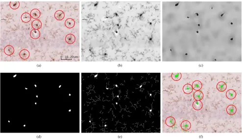
Noise is inherent in histology images. Research for quantitat-ive analysis of microglial often relies on thresholding (manual or automatically) [20], [21], [31]. These methods are not suitable for dealing with noisy and inhomogeneous histological images of microglia. A preprocessing step is therefore needed to remove noise whilst preserving the details of microglia in the image. An adaptive thresholding algorithm, which automatically determines threshold values for different parts of the image, is then applied to the denoised images to extract the microglia. Tiny microglia with a soma size smaller than 16.7µm are also removed, as suggested in [20]. In Alzheimer’s Disease, clusters of microglia with the morphological appearance of an activated phenotype are found around amyloid plaques [32]. These clusters are detected by their abnormal soma sizes and analysed separately. Finally, the segmented microglia processes are skeletonised and combined with the segmented microglia soma, and the isolated microglial processes, not connected to any microglia soma, are removed. Figure 1 shows the workflow of the proposed segmentation method.
Denoising with Mumford-Shah Total Variation: Our previous research [25], [26], [33] has shown that the classical variational Mumford-Shah model [22], [24] that uses a total variation regulariser (named as MSTV model in this paper) [23] is fast and accurate and is therefore chosen to denoise microglia images. The MSTV model can smooth microglia images and preserve the edges of objects, making it easier to detect microglia in the image. Furthermore, MSTV can benefit from fast imaging solvers such as the FFT and shrinkage, which
makes it very efficient to implement. The MSTV model works as follows [24],
Eε(u, v) = Z
Ω
(u−f)2dx
+α
Z
Ω
v2|∇u|dx
+β
Z
Ω
ε|∇v|2+(v−1) 2
4ε
!
dx
(1)
whereα,β andεare three positive parameters balancing the energy terms;uis a piecewise smooth function to approximate the original imagef; andv is a piecewise smooth function to represent object edges in the image (v takes value 0 on the edges and 1 in smooth regions). This energy functional can be used to smooth the image as well as find the edges of objects in the image.
A fast split Bregman algorithm [27] is designed for discret-ising and solving the MSTV model equations. This algorithm has been widely used to solve L1-based variational models [34], [35], [36], [28], [29], [30]. An auxiliary vectorw= (w1, w2)
and a Bregman iteration parameter b= (b1, b2)are introduced
to transform the minimisation of the MSTV model into optimising energy functional, as follows:
Eε(u, v, w) = Z
Ω
(u−f)2dx+α
Z
Ω
v2|w|dx
+θ 2
Z
Ω
(w− ∇u−b)2dx
+β
Z
Ω
ε|∇v|2+(v−1) 2
4ε
!
dx
(2)
whereθis positive penalty parameter. In practice, each variable
u,w andv in functional (2) is solved separately, for example, variablesv andw fixed first, and the Euler-equation ofuis solved as follows,
u+θ∆u=f+θdiv wk−bk
(3)
where div and ∆ denote divergence operator and Laplace operator respectively, andk stands for the current number of iterations. By applying discrete Fourier transform to both sides of the equation, the closed-form solution of uis obtained,
uk+1=< F−1 F(f) +θF(div)F w k−bk
1 +θF(∆)
!!
(4)
whereF(·)andF−1(·)denotes the discrete Fourier transform
and inverse Fourier transform respectively. <(·) is the real part of a complex number,0−0 stands for pointwise division of matrices. The minimization with respect towcan be expressed as follows,
wk+1=
argmin w∈R4
E(w) =α
Z
Ω
v2|w|dx+θ 2
Z
Ω
(w− ∇u−b)2dx
(5)
It is easy to check that,
wk+1= max
∇uk+1+bk −
α θv
2,0 ∇uk+1+bk
(a) (b) (c)
[image:3.612.61.555.63.347.2](d) (e) (f)
Figure 1. Workflow of the proposed segmentation for a sample image (a) Original histology image (b) Smoothed image (α=10) (c) Smoothed image (α=300) (d) Soma segmentation (e) Soma and processes segmentation (f) Automatically labelled microglia overlaid onto histological image. Inclusion criteria: soma size larger than 16.7µm.
with the convention0/0 = 0.
The above equation is known as the analytical soft threshold-ing equation or shrinkage. Note that shrinkage (3) includes two subshrinkages for each component of vector w. The solution of the Euler-Lagrange equation of v with theuandwfixed is obtained as follows,
2αvwk+1
−2βε∆v+β (v−1)
2ε = 0 (7)
This equation can be efficiently solved by one iteration of Gauss-Seidel. Finally, the parameter is updated using
bk+1=bk+∇uk+1−wk+1 (8)
The parameters α,θ,β andεin (2) can be adjusted.αis a smoothing parameter and larger αgives smoother result. We set α=10 as a weak smooth andα=300 as a strong smooth. The selection of α was based on the results of a series of experiments using different smoothing values on microglial images. Figure 2 shows example results of a single microglial cell that was smoothed using different α values. It can be seen that the method produced the best results whenα=10 and
α=300 were chosen for, removing noise, and simultaneously preserving the details of microglial cell body and processes in the images respectively.
Due to the Bregman iteration technique used, different pen-alty parameter θwill provide similar smooth result. However, the algorithm may have different rate of convergence with different values of θ. In all the experiments, the value of
θ is fixed as 5 in order to achieve a fast convergence rate.
(a) (b) (c) (d)
(e) (f) (g) (h)
Figure 2. Smoothed microglial cell (a)α=0 (b)α=10 (c)α=20 (d)α=30 (e) α=100 (f)α=200 (g)α=300 (h)α=400.
Parameterβ balances the last energy term against the other three terms in model (2). It is empirically chosen as 0.1 for all experiments. The approximation of Mumford-Shah regulariser term in the proposed model (i.e. the last two energy term in (1)) is based on the phase field approach underγ-convergence [37]. Theoretically, parameterεshould be close enough to zero to satisfy such approximation. Therefore, we setε= 0.0001
for all the experiments.
B. Feature Extraction
[image:3.612.329.551.409.545.2](a) (b)
[image:4.612.62.555.69.501.2](c) (d)
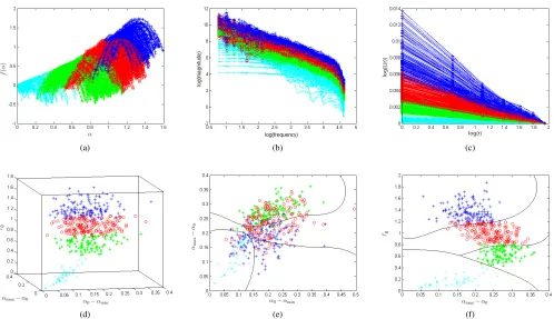
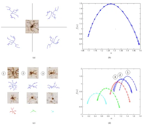
Figure 3. Multifractal spectra of microglia. (a) Segmented microglia rotated in four different directions (b) Multifractalα/f(α)spectra of the microglia. (c) Segmented microglia in four common activation states (d) Multifractalα/f(α)spectra. Ramified (Blue): resting (1) and intermediate (2,3). Partially ramified (Red): bushy. Slightly ramified (Green). Activated (Cyan): amoeboid.
to extract features from microglia. A major concept in fractal analysis of a structure is fractal dimension D, which can be defined in different ways depending on the measure with which the scaling law is determined. The simplest is the box-counting dimension, where the measure is the box that contains at least a point of the fractal structure, and the scaling law is
N(s) = lim s→0s
−D, where N(s) is the minimum number of
boxes needed to cover the structure, s is the monotonically decreasing size of the box, andD is the fractal dimension of the structure.
Rather than calculating a single fractal dimension value, multifractal analysis [38], [39] produces a fractal spectrum
D(h) for the fractal structure, consisting of a set of fractal dimensions, each of which measures the dimension of the set of points on the structure with the same H¨older exponent value
h. The H¨older exponent is the supremum of allh∈(n, n+ 1)
that satisfy the following condition:
|f(x)−Pn(x−x0)| ≤C|x−x0|h (9)
where f is a function;xis a point in the neighbourhood of
x0; C is a constant; andPn is a polynomial of degreen < h.
Effectively, the H¨older exponent of a function f at a point characterises the regularity of f at that point.
The multifractal spectrum D(h) is a function of H¨older exponenth. In the literature the H¨older exponent is commonly represented as α, and the corresponding multifractal spectrum
(a) (b)
Figure 4. (a) Fourier power spectra in log-log scale and (b) lacunarity plot of the microglia in Figure 3 in four common activation states. Ramified (Blue): resting (1) and intermediate (2,3). Partially ramified (Red): bushy. Slightly ramified (Green). Activated (Cyan): amoeboid.
behaviour of the partition functionZ:
Z(q, s) = (X i
µqi(s))∼sτ(q) (10)
f(α) =qα(q)−τ(q) (11)
where the variables q and τ(q) play the same role as the inverse of temperature and free energy in thermodynamics; the Legendre transform (11) indicates that α and f(α) are the thermodynamical conjugate to q and τ(q); and τ(q) = (q−1)Dq,α(q)∼=dτd(qq).
Figure 3b shows multifractal spectra of the same microglia image rotated in eight directions. It is clear that the fractal spectra for all the images are the same. Orientation invariant is one of the advantages of multifractal analysis, as the same structure may appear in different orientations in images and image analysis methods should be robust to these orientation variations. In general, the more complex and ramified the microglia’ structure, the larger the fractal dimension, and the wider the multifractal spectrum, the denser the microglia’ structure. The spectrum can be left or right skewed or symmetrical when αmax−α0 and α0 −αmin are equal, α0
is where the spectrum reaches its maximum. Experiments show that these characteristics of the multifractal spectrum can be used to distinguish microglia in different activation states. Figure 3c and Figure 4b show microglia in four activation states and their fractal spectra: Ramified (resting and intermediate), partially ramified (bushy), slightly ramified and activated (amoeboid). The spectra of microglia images in different activation states are distinct. However, for some images, these features are not discriminative enough, which means that these features alone are not sufficient to describe the local variations of the microglia. To improve classification accuracy, further information about the microglia image is needed.
Fourier Fractal Features: We first resort to the Fourier transform to extract additional information about the structure in the frequency domain. Recall that when calculating fractal
dimension using the box counting method, the number of boxes N needed to cover a structure and the size s of the box obey the power law, and fractal dimension is the slope of the log-log plotlog(N)on the Y-axis against log(s) on the X-axis. A steeper slope means that the microglia’ structure is less ramified. According to [42], the Fourier power spectrum (FPS) of a grayscale image and spatial frequency (f) also obey the power law. This provides another way to calculate fractal dimension, using the Fourier transform. The Fourier fractal dimension (FFD) can be defined as the slope of the log-log plot oflog(F P S)on the Y-axis against log(f)on the X-axis. In practice, the Fourier fractal dimension (FFD) is defined as:
F F D= 6 +β
2 (12)
whereβ is the slope of the least square line fitted to the Fourier power spectrum in log-log scale.
Example plots oflog(F P S)of images againstlog(f)are shown in Figure 4a. Because binary microglia images are used for the experiments and the Fourier power spectra and spatial frequency slightly deviate from the power law. This has also been reported in [43]. However, the plots of microglia images in different activation states are still quite distinct, especially at high frequencies.
Lacunarity Features: Further more, lacunarity, which de-scribes the heterogeneity of fractal structures, complements fractal dimension by measuring how the data fills the space [11]. A box-counting algorithm is used for estimating lacunarity [44]. The algorithm uses a unit box of size r to glide over the entire image. The number of points within the box (mass
p) is counted at each step and a distribution of box masses
B(p, r)is created at the end of gliding. The distribution is then converted into a probability distribution Q(p, r)by dividing the total number of boxesB(r)of sizer:
Q(p, r) =B(p, r)
[image:5.612.71.550.72.271.2]Lacunarity is then defined as the division of first and second moments of the box mass probability distribution:
L(r) = P
ppQ(P, r)
P
pp2Q(P, r)
2 (14)
Figure 4b shows example lacunarity plots of microglia in different states. The plots of microglia images in different activation states are distinct at small scales (box size), more ramified microglia has higher lacunarity values than less ramified microglia as it is ”less rotationally invariant”. This is in agreement with the results in [11].
In summary, in this paper, the features extracted from the microglia for classification are the multifractal features (the peak of the multifractal spectrum (f0) and the symmetry features αmax−α0 and α0−αmin), lacunarity value at the smallest scale (Lmin) as well as the Fourier features (FFD
and the FPS magnitude values at high frequencies), and these features together are named the combinatory feature.
III. EXPERIMENTALVALIDATION OFMETHODS
A. Data Acquisition
The data used in this paper were generated from brain tissue from female mice, transgenic APPswe/PS1dE9, a mouse model of Alzheimer’s disease, or their wild-type littermate. All mice were were bred in the University of Nottingham’s Biomedical Service Unit as previously described [45]. Some of these mice had been treated 10 days before with a lipopolysaccharide im-mune challenge (LPS, 100ug/kg) known to selectively activate microglia or its vehicle Phosphate Buffered Saline (PBS, Sigma Aldrich, St. Louis, MO, USA). The genotype and treatment condition ensured a wider representation of morphological states but were not analysed systematically as the focus on the paper is on classification. All procedures were approved as required under the UK Animals (Scientific Procedures) Act 1986. Brains were fixed in 4% Paraformaldehyde for at least 24 hours at 4◦C and embedded in paraffin wax on a tissue embedding station (Leica TP1020). 7µm-thick coronal sections were cut throughout the hippocampus using a microtome, mounted on 3-Aminopropyltriethoxysilane-coated slides and dried overnight at 40◦C. Immunostaining was carried out using standard procedures at room temperature, as described below. All the solutions were freshly prepared using PBS + 1% Tween 80, except DAB solution that was prepared in distilled water. Briefly, the tissue was re-hydrated in consecutive rinses in Xylene, 100% ethanol, 70% ethanol and distilled water. Antigen retrieval was performed by 20 minutes incubation in Sodium Citrate buffer at 95-99◦C, followed by incubation in 1% H2O2 (Sigma Aldrich, St. Louis, MO, USA). Tissue was then blocked in 5% normal goat serum (Vector Laboratories, Burlingame, CA), incubated in rabbit polyclonal anti-Iba-1 primary antibody (anti-Iba-1:6000; WAKO Chemicals, VA, USA) for 1 hour followed by 30 minutes incubation with anti-rabbit secondary antibody (1:200; Vector Laboratories Inc. Burlingame, CA). After washing, sections were incubated with Vectastain Elite ABC kit (Vector Laboratories Inc. Burlingame, CA) and labelled with DAB peroxidase substrate (Vector
Laboratories, Burlingame, CA) according to manufacturer’s instructions. To reveal histologic morphology, sections were then lightly counterstained with haematoxylin (purplish-blue nuclear stain) and eosin (pink cytoplasmic stain) and mounted with DPX-mount media.
Digital focused photo-scanning images were acquired using a Hamamatsu NanoZoomer-XR with TDI camera technology at a magnification of 20X. Rectangular regions of interest (ROIs) were drawn within the hippocampus subfields with an area of 0.2 mm2 or 0.1mm2 using NDP.view2.
B. Validation of Segmentation Method
Previous studies have identified the limitations of the existing microlia segmentation methods [16]. This includes: microglia contrast issues within the same image, large artifacts, different visual textures within the same field of view and textures that blur the distinction between microglia cell and background. Experiments show that the proposed segmentation method is accurate and overcomes these problems. Some example segmentation results are shown in Figure 5.
(a) (b) (c) (d)
[image:7.612.51.567.64.354.2](e) (f) (g) (h)
Figure 5. Challenges described in [16] and the proposed method overcomes these problems (a) Image shows microglia cells with strong and weak intensities (b) Image has a large complex artifact with microglia located partly inside the artifact (c) image shows two regions that exhibit different visual textures (d) Image displays a complex texture appearance that blurs the distinction between microglia cell and background pixels. (e) (h) Microglia soma labelled using the proposed method.
(a) (b) (c)
(d) (e) (f)
[image:7.612.54.567.421.670.2](a) (b)
[image:8.612.54.567.64.416.2](c) (d) (e)
Figure 7. Comparison of segmentation results using the proposed segmentation method and the manual segmentation method. (a) Microglia soma segmented using the proposed automatic segmentation method. (b) Microglia soma manually segmented by an expert. Analysis results calculated using automatic and manual segmentation methods within the hippocampus. (c) Soma number (d) Soma area. ***, p¡0.0001. Statistically significant differences between scorers and between some scorers and automated method (e) Percent area stained. **, p¡0.01. ***, p¡0.0001. Statistically significant differences between scorers and between scorers and automated method. Automatic: results produced by the proposed method. Manual A and Manual B: results produced by the experts. Data are presented as means + standard error.
(a) (b) (c) (d)
Figure 8. Artifacts that the both the thresholding and proposed method incorrectly detected as microglia and which can be manually unselected with the proposed metthod.
C. Feature Extraction
To evaluate the performance of the extracted multifractal features for classification, 500 microglia are first extracted from a selected histology image and divided into four groups based on their morphologies. Multifractal analysis is performed
[image:8.612.56.577.499.638.2](a) (b) (c)
[image:9.612.59.557.68.355.2](d) (e) (f)
Figure 9. Multifractal analysis of microglia in four common activation states (a) Multifractalα/f(α)spectra (b) Fourier power spectra in log-log scale. (c) Lacunarity/box size plot. (d) Feature of the multifractal spectra in (a)α0−αmin−/αmax−α0 /f0 (e) Feature of the multifractal spectraα0−αmin−
/αmax−α0 (f) Feature of the spectra in (a)αmax−α0 /f0. The boundary curve (by SVM classifier) show clear difference between four classes.
Number of Features Feature Descriptions Feature Names Accuracy
Mono Fractal Features
1 Peak of Multifractal Spectrum f0 93.17%
1 Slop of Fourier Power Spectrum FFD 45.62%
1 Lacunarity Value (at Minimum Scale) Lmin 90.32%
Multi Fractal Features
3 Combination of Three Mono Fractal Features f0+ FFD+Lmin 93.15%
3 Peak of Multifractal Spectrum+ Symmetry Feature f0+α0−αmin+αmax−α0 91.08%
4 Peak of Multifractal Spectrum+ Symmetry Feature, Lacunarity Value
f0+α0−αmin+αmax−α0+
Lmin 93.92%
4 Slop of Fourier Power Spectrum+
Fourier Power Spectrum Magnitude Values at High Frequencies FFD+FPS feature 86.25%
8 Combinatory Fractal Features f0+α0−αmin+αmax−α0+
Lmin+ FFD+ FPS feature 94.27%
Gabor
Features 40
Gabor Features Extracted
From Greyscale Microglia Image Gabor Features 21.65% Table I
CLASSIFICATION ACCURACY WITHSVMON DIFFERENT FEATURES.
the plots are colour coded to represent the different activation states of the microglia. It can be seen that the plots of the four classes are separated. Figure 9d, Figure 9e and Figure 9f show that the plot of four classes using three features is more discriminate than the plots using two features. The results indicate there is a good ground for automated classification of the microglia using the extracted fractal features.
D. Classification
To evaluate the performance of the proposed feature extrac-tion methods for classificaextrac-tion, a non-linear Support Vector Machine (SVM) classifier with Gaussian Radial Basis Function (RBF) kernel [47] is chosen for classification of the extracted microglia features. The SVM classifies data by finding an optimal hyperplane that separates data points of one class
from those of the other class. The position of the hyperplane is defined by a small subset of data that lies closest to the decision surface, and these points are known as support vectors. The best hyperplane for an SVM is the one with the largest margin between the two classes, where margin is the distance from the decision surface to the support vectors.
The dataset is split into half, one as training set and one test set, each containing an equal number of microglia images in different activation states. The classifier is trained using the training set and tested using the test set. The process is repeated 100 times and results are averaged. The classification results are shown in Table I. Results show that SVM performed poorly on monofractal dimension features (f0, FFD, Lmin)
(a) (b)
(c) (d)
[image:10.612.91.530.66.581.2](e) (f)
Figure 10. Analysis results of a typical (a) Alzheimer’s mouse brain slice (b) healthy mouse brain slice (c)(d) Zoomed in hippocampal regions of the images in (a)(b) respectively. Microglia are labelled in five different colours. Cyan: activated, Green: slightly ramified, Red: partially ramified. Blue: fully ramified, Yellow: Clusters or artifacts. (e)(f) Heat map of the microglia density image and the corresponding colour bar, representing the number of microglia within a square region.
Performance of features extracted from the original microglia images was also evaluated and compared with the proposed methods using multifractal features. Gabor wavelets were applied directly to the grayscale microglia images. Results show that SVM performed poorly using the features from the microglia images. This is because the classification is affected by the orientation of the microglia and the illumination of the images. In contrast, the proposed methods using multifractal
features have produced good classification accuracy.
In this paper, automated image analysis methods are intro-duced for segmenting the microglia from histology images and analysing their morphology. Segmentation of both microglia process and soma is achieved through a novel variational method in combination with a fast split Bregman algorithm which overcomes the problems caused by inhomogeneity of histology images. Analysis of microglia activation states is achieved through SVM classification of a combination of multifractal features extracted from the microglia. Experiments show that the proposed methods are accurate, thus eliminating the inter-rater variability seen with manual analysis, and scalable to analysing large microglial datasets. To the best of our knowledge, this is the first time that multifractal analysis is used to extract features for classifying microglial activation states. For future work, the microglia segmentation and analysis framework described in this paper will be tested on large histology datasets of healthy and diseased brains, along with ground truth images, to validate its sensitivity to disease progression and pro-inflammatory states and therefore a viable tool for studying microglial biology.
REFERENCES
[1] L. Lawson, V. Perry, and S. Gordon, “Turnover of resident microglia in the normal adult mouse brain,”Neuroscience, vol. 48, no. 2, pp. 405–415, 1992.
[2] A. J. Dowding, A. Maggs, and J. Scholes, “Diversity amongst the microglia in growing and regenerating fish cns: Immunohistochemical characterization using fl. 1, an anti-macrophage monoclonal antibody,”
Glia, vol. 4, no. 4, pp. 345–364, 1991.
[3] X.-G. Luo and S.-D. Chen, “The changing phenotype of microglia from homeostasis to disease,”Transl Neurodegener, vol. 1, no. 9, 2012. [4] B. Faith, “Microglia: A standing ovation, please!,”Brain Sense, 2011. [5] L. R. Frick, K. Williams, and C. Pittenger, “Microglial dysregulation in
psychiatric disease,”Journal of Immunology Research, vol. 2013, 2013. [6] J. Vinet, H. Weering, A. Heinrich, R. E. K¨alin, A. Wegner, N. Brouwer, F. L. Heppner, N. v. Rooijen, H. Boddeke, and K. Biber, “Neuropro-tective function for ramified microglia in hippocampal excitotoxicity,”J Neuroinflammation, vol. 9, no. 1, p. 27, 2012.
[7] L. R. Watkins, E. D. Milligan, and S. F. Maier, “Glial activation: a driving force for pathological pain,”Trends in neurosciences, vol. 24, no. 8, pp. 450–455, 2001.
[8] P. Kapeller, S. Ropele, C. Enzinger, T. Lahousen, S. Strasser-Fuchs, R. Schmidt, and F. Fazekas, “Discrimination of white matter lesions and multiple sclerosis plaques by short echo quantitative 1hmagnetic resonance spectroscopy,”Journal of neurology, vol. 252, no. 10, pp. 1229– 1234, 2005.
[9] D. Z´adori, G. Nyiri, A. Sz˝onyi, I. Szatm´ari, F. F¨ul¨op, J. Toldi, T. F. Freund, L. V´ecsei, and P. Kliv´enyi, “Neuroprotective effects of a novel kynurenic acid analogue in a transgenic mouse model of huntingtons disease,”Journal of neural transmission, vol. 118, no. 6, pp. 865–875, 2011.
[10] H. Akiyama, S. Barger, S. Barnum, B. Bradt, J. Bauer, G. M. Cole, N. R. Cooper, P. Eikelenboom, M. Emmerling, B. L. Fiebich,et al., “Inflammation and alzheimers disease,”Neurobiology of aging, vol. 21,
no. 3, pp. 383–421, 2000.
[16] N. A. Valous, B. Lahrmann, W. Zhou, R. Veltkamp, and N. Grabe, “Multistage histopathological image segmentation of iba1-stained murine microglias in a focal ischemia model: Methodological workflow and expert validation,” Journal of neuroscience methods, vol. 213, no. 2, pp. 250–262, 2013.
[17] L. A. Cysique, K. Moffat, D. M. Moore, T. A. Lane, N. W. Davies, A. Carr, B. J. Brew, and C. Rae, “Hiv, vascular and aging injuries in the brain of clinically stable hiv-infected adults: a 1h mrs study,”PloS one, vol. 8, no. 4, p. e61738, 2013.
[18] H. Jelinek, A. Karperien, A. Buchan, and T. Bossomaier, “Differenti-ating grades of microglia activation with fractal analysis,”Complexity International, vol. 12, 2008.
[19] D. J. Donnelly, J. C. Gensel, D. P. Ankeny, N. van Rooijen, and P. G. Popovich, “An efficient and reproducible method for quantifying macrophages in different experimental models of central nervous system pathology,”Journal of neuroscience methods, vol. 181, no. 1, pp. 36–44, 2009.
[20] C. Kozlowski and R. M. Weimer, “An automated method to quantify microglia morphology and application to monitor activation state longitudinally in vivo,”PloS one, vol. 7, no. 2, p. e31814, 2012. [21] I. B. Hovens, C. Nyakas, R. G. Schoemaker,et al., “A novel method for
evaluating microglial activation using ionized calcium-binding adaptor protein-1 staining: cell body to cell size ratio,”Neuroimmunology and Neuroinflammation, vol. 1, no. 2, p. 82, 2014.
[22] D. Mumford and J. Shah, “Optimal approximations by piecewise smooth functions and associated variational problems,”Communications on pure and applied mathematics, vol. 42, no. 5, pp. 577–685, 1989.
[23] L. I. Rudin, S. Osher, and E. Fatemi, “Nonlinear total variation based noise removal algorithms,”Physica D: Nonlinear Phenomena, vol. 60, no. 1, pp. 259–268, 1992.
[24] J. Shah, “A common framework for curve evolution, segmentation and anisotropic diffusion,” in Computer Vision and Pattern Recognition, pp. 136–142, IEEE, 1996.
[25] J. Duan, C. Tench, I. Gottlob, F. Proudlock, and L. Bai, “New variational image decomposition model for simultaneously denoising and segmenting optical coherence tomography images,”Physics in medicine and biology, vol. 60, no. 22, pp. 8901–8922, 2015.
[26] J. Duan, Y. Ding, Z. Pan, J. Yang, and L. Bai, “Second order mumford-shah model for image denoising,” in Image Processing (ICIP), 2015 IEEE International Conference on, pp. 547–551, IEEE, 2015. [27] T. Goldstein and S. Osher, “The split bregman method for l1-regularized
problems,”SIAM Journal on Imaging Sciences, vol. 2, no. 2, pp. 323–343, 2009.
[28] J. Duan, Z. Qiu, W. Lu, G. Wang, Z. Pan, and L. Bai, “An edge-weighted second order variational model for image decomposition,”Digital Signal Processing, vol. 49, pp. 162–181, 2016.
[29] W. Lu, J. Duan, Z. Qiu, Z. Pan, R. W. Liu, and L. Bai, “Implementation of high-order variational models made easy for image processing,”
Mathematical Methods in the Applied Sciences, 2016.
[30] J. Duan, W. Lu, C. Tench, I. Gottlob, F. Proudlock, N. N. Samani, and L. Bai, “Denoising optical coherence tomography using second order total generalized variation decomposition,”Biomedical Signal Processing and Control, vol. 24, pp. 120–127, 2016.
[31] Z. Sołtys, M. Ziaja, R. Pawli´nski, Z. Setkowicz, and K. Janeczko, “Morphology of reactive microglia in the injured cerebral cortex. fractal analysis and complementary quantitative methods,”Journal of neuros-cience research, vol. 63, no. 1, pp. 90–97, 2001.
[32] T. Wyss-Coray and J. Rogers, “Inflammation in alzheimer diseasea brief review of the basic science and clinical literature,”Cold Spring Harbor perspectives in medicine, vol. 2, no. 1, p. a006346, 2012.
[33] J. Duan, W. Lu, Z. Pan, and L. Bai, “New second order mumford-shah model based onγ-convergence approximation for image processing,”
[34] J. Duan, Z. Pan, X. Yin, W. Wei, and G. Wang, “Some fast projection methods based on chan-vese model for image segmentation,”EURASIP Journal on Image and Video Processing, vol. 2014, no. 1, pp. 1–16, 2014.
[35] J. Duan, C. Tench, I. Gottlob, F. Proudlock, and L. Bai, “Optical coherence tomography image segmentation,” inImage Processing (ICIP), 2015 IEEE International Conference on, pp. 4278–4282, IEEE, 2015. [36] J. Duan, Z. Pan, B. Zhang, W. Liu, and X.-C. Tai, “Fast algorithm for
color texture image inpainting using the non-local ctv model,”Journal of Global Optimization, pp. 1–24, 2015.
[37] L. Ambrosio and V. M. Tortorelli, “Approximation of functional depend-ing on jumps by elliptic functional via t-convergence,”Communications on Pure and Applied Mathematics, vol. 43, no. 8, pp. 999–1036, 1990. [38] W. O. C. Ward and L. Bai, “Multifractal analysis of microvasculature in health and disease,” in35th Annual International Conference of the IEEE on Engineering in Medicine and Biology Society, pp. 2336–2339, 2013.
[39] Y. Ding, W. Ward, J. Duan, D. Auer, P. Gowland, and L. Bai, “Retinal vasculature classification using novel multifractal features,”Physics in Medicine and Biology, 2015.
[40] A. Arneodo, B. Audit, N. Decoster, J.-F. Muzy, and V. C,The Science of Disasters - Wavelet based multifractal formalism: Applications to DNA sequences, satellite images of the cloud structure and stock market data. Springer, 2002.
[41] A. Arneodo, E. Bacryb, and J. F. Muzya,The thermodynamics of fractals revisted with wavelets. Cambridge University Press, 2004.
[42] J. C. Russ,Fractal surfaces. Springer, 1994.
[43] T. Melmer, S. A. Amirshahi, M. Koch, J. Denzler, and C. Redies, “From regular text to artistic writing and artworks: Fourier statistics of images with low and high aesthetic appeal,”Frontiers in human neuroscience, vol. 7, 2013.
[44] C. R. Tolle, T. R. McJunkin, and D. J. Gorsich, “An efficient implement-ation of the gliding box lacunarity algorithm,”Physica D: Nonlinear Phenomena, vol. 237, no. 3, pp. 306–315, 2008.
[45] C. Bonardi, F. de Pulford, D. Jennings, and M.-C. Pardon, “A detailed analysis of the early context extinction deficits seen in appswe/ps1de9 female mice and their relevance to preclinical alzheimer’s disease,”
Behavioural brain research, vol. 222, no. 1, pp. 89–97, 2011. [46] C. A. Schneider, W. S. Rasband, and K. W. Eliceiri, “Nih image to
imagej: 25 years of image analysis,”Nature methods, vol. 9, no. 7, pp. 671–675, 2012.
[47] B. Scholkopf, K.-K. Sung, C. J. Burges, F. Girosi, P. Niyogi, T. Poggio, and V. Vapnik, “Comparing support vector machines with gaussian kernels to radial basis function classifiers,”IEEE Transactions on Signal Processing, vol. 45, no. 11, pp. 2758–2765, 1997.
[48] M.-C. Pardon, M. Y. Lopez, D. Yuchun, M. Marja´nska, M. Prior, C. Brignell, S. Parhizkar, A. Agostini, L. Bai, D. P. Auer, et al., “Magnetic resonance spectroscopy discriminates the response to microglial stimulation of wild type and alzheimers disease models,” Scientific reports, vol. 6, 2016.
[49] A. Agostini, Y. Ding, L. Bai, and M. C. Pardon, “Unaltered susceptibility to neuroinflammation in pre-symptomatic appswe/ps1e9 mice, focus on genotype and sex differences,” inMeeting of the British Association for Psychopharmacology, 2015.
Yuchun Ding received B.Sc. (2011) in computer science from the University of Nottingham. During 2011-2012, he was a software engineer for the development of a SCADA system in Willowglen MSC Berhad. He then joined the University of Nottingham and received Ph.D. in computer science in 2016. He is currently a post-doctoral researcher in the University of Newcastle, computing science department. His research interests include medical image analysis and digital pathology.

![Figure 5. Challenges described in [16(b) Image has a large complex artifact with microglia located partly inside the artifact (c) image shows two regions that exhibit different visual textures (d)] and the proposed method overcomes these problems (a) Image](https://thumb-us.123doks.com/thumbv2/123dok_us/8599581.372291/7.612.54.567.421.670/challenges-described-artifact-microglia-different-proposed-overcomes-problems.webp)