Controls on the transport of oceanic heat to Kangerdlugssuaq Glacier, East Greenland

Controls on the transport of oceanic heat to Kangerdlugssuaq

Glacier, East Greenland

TOM COWTON,

ANDREW SOLE,

PETER NIENOW,

DONALD SLATER,

DAVID WILTON,

EDWARD HANNA

1_{School of Geosciences,University of Edinburgh,Drummond Street,Edinburgh,EH10 4ET,UK}

2_{Department of Geography and Sustainable Development,University of St Andrews,St Andrews,KY16 9AL,UK} 3_{Department of Geography,University of Sheffield,Winter Street,Sheffield,S10 2TN,UK}

Correspondence Tom Cowton_<tom.cowton@st-andrews.ac.uk_>

ABSTRACT. Greenland’s marine-terminating glaciers may be sensitive to oceanic heat, but the fjord pro-cesses controlling delivery of this heat to glacier termini remain poorly constrained. Here we use a three-dimensional numerical model of Kangerdlugssuaq Fjord, East Greenland, to examine controls on fjord/ shelf exchange. We find that shelf-forced intermediary circulation can replace up to∼25% of the fjord volume with shelf waters within 10 d, while buoyancy-driven circulation (forced by subglacial runoff from marine-terminating glaciers) exchanges ∼10% of the fjord volume over a 10 d period under typical summer conditions. However, while the intermediary circulation generates higher exchange rates between the fjord and shelf, the buoyancy-driven circulation is consistent over time hence more efficient at transporting water along the full length of the fjord. We thus find that buoyancy-driven cir-culation is the primary conveyor of oceanic heat to glaciers during the melt season. Intermediary circu-lation will however dominate during winter unless there is sufficient input of fresh water from subglacial melting. Our findings suggest that increasing shelf water temperatures and stronger buoyancy-driven cir-culation caused the heat available for melting at Kangerdlugssuaq Glacier to increase by∼50% between 1993–2001 and 2002–11, broadly coincident with the onset of rapid retreat at this glacier.

KEYWORDS:arctic glaciology, calving, glacier discharge, ice/ocean interactions

1. INTRODUCTION

Many of Greenland’s marine-terminating outlet glaciers underwent a phase of rapid retreat and acceleration in the late 1990s and early 2000s (Rignot and Kanagaratnam, 2006), with the consequent discharge of ice into the ocean re-sponsible for 58% of total mass loss from the ice sheet over the period 2000–05 (Enderlin and others,2014). This retreat was coincident with a period of ocean warming around Greenland (e.g. Hanna and others,2009; Rignot and others, 2012), leading to suggestions that retreat may have been trig-gered by increased submarine melting at the calving fronts of marine-terminating glaciers (e.g. Straneo and Heimbach, 2013). These glaciers are however typically separated from the shelf by long, narrow fjords, which modulate the delivery of oceanic heat to the ice-sheet margins (Straneo and Cenedese,2015). Until the processes controlling fjord circula-tion are better understood and quantified, the timescales on which marine-terminating outlet glaciers may be sensitive to variability in ocean temperature remain difficult to assess. A lack of understanding of fjord processes also hinders our ability to quantify the exchange of heat and fresh water between the ocean and the ice sheet, and to predict how this exchange will evolve as the climate warms.

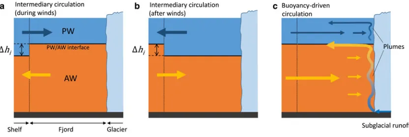
Two mechanisms have been proposed as the primary drivers of exchange between the fjord and shelf, and thereby delivery of oceanic heat to glacier termini (e.g. Straneo and Cenedese,2015). In the first mechanism ( inter-mediary circulation), the exchange is driven by density gradi-ents, which form between the fjord and shelf as a result of variability in shelf water properties, particularly during the

passage of coastal storms (e.g. Arneborg,2004; Jackson and others,2014). In the second mechanism (buoyancy-driven circulation), the input to the fjord of meltwater runoff (and to a lesser extent fresh water from submarine melt) from glaciers drives exchange. The relative efficacy of these processes, and how they may differ between fjords and over time, remains poorly understood (Straneo and others,2013).

transport of oceanic heat towards Kangerdlugssuaq Glacier (KG) between 1993 and 2012.

2. SETTING

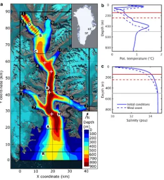
KF is more than 60 km long, between 5 and∼20 km wide (de-pending on the defined location of the mouth) and up to∼900 m deep (Fig. 1a). It forms the main trunk of a system containing four further tributary fjords. KF connects with Kangerdlugssuaq Trough, which provides a relatively deep (>400 m) pathway between the fjord and the continental shelf break (Christoffersen and others,2011). KG, which drains into the head of KF, is the largest outlet glacier on Greenland’s east coast, responsible for∼5% of ice discharge from Greenland (Enderlin and others,2014). Like many of the glaciers along the southeast coast of Greenland, KG has undergone substan-tial dynamic change since the 1990s, most notably between summer 2004 and spring 2005, when the terminus retreated by 7 km and accelerated from 7.3 to 13.9 km a−1 (Howat and others 2007; Luckman and others, 2006). This retreat

was broadly coincident with an increase in subsurface ocean temperature off southeast Greenland (Hanna and others, 2009; Rignot and others, 2012), driven by an anomalous inflow of relatively warm, salty subtropical Atlantic water (AW) into the subpolar North Atlantic (Straneo and Heimbach,2013). Around the coast of Greenland, this AW is overlain by cooler, fresher polar water (PW). Hydrographic observations from KF and Sermilik Fjord (SF, another large fjord in southeast Greenland) show a strong two layer stratifica-tion, demonstrating that AW is able to access these deep fjords (Christoffersen and others, 2011; Straneo and others, 2011, 2012; Jackson and others, 2014; Sutherland and others, 2014), though the processes controlling the exchange of waters between the shelf and fjord remain poorly constrained (Straneo and Heimbach,2013).

Based on the temperature and salinity data used for the initial conditions (Section 3.3;Figs 1b,c), the Rossby deform-ation radius (e.g. Garvine,1995) of KF is ∼10 km. As such, while significant across-fjord variability is not expected throughout much of the fjord’s length, rotational dynamics

may become significant in the broader zones up-fjord of section C and, more notably, between sections A and M at the fjord mouth (Fig. 1a). A thorough analysis of the estuarine dynamics of KF was undertaken by Sutherland and others (2014), on the basis of hydrographic observations obtained during August 2009. Their results indicated that KF is a highly stratified fjord system in which freshwater forcing (from glacial runoff) and tidal currents are weak and only the strongest along-fjord winds can generate a significant over-turning circulation (Sutherland and others,2014). However, as identified by Sutherland and others (2014), an analysis of conventional estuarine parameter space may not be appropri-ate for KF. Two features stand out: firstly, intermediary circula-tion, due to variation in shelf water stratificacircula-tion, may be a key driver of fjord-shelf exchange, and secondly, the input of glacial meltwater runoff at depth (i.e. subglacially) may signifi-cantly modify the freshwater forcing effect on the fjord relative to an equivalent input of runoff at the surface. These features are investigated further in this study.

3. METHODS

3.1. Model

Our model simulations are run using MITgcm (Adcroft and others, 2004), a versatile finite-volume circulation model that has been used in numerous studies of interaction between the ocean and ice masses (e.g. Losch, 2008; Xu and others, 2012; Sciascia and others, 2014). Plumes arising from the subglacial input of meltwater are parame-terised using a coupled plume model (Cowton and others, 2015), which uses buoyant plume theory (Morton and others, 1956; Jenkins, 2011) to simulate a plume of half-conical form based on the stratification of the fjord and the prescribed meltwater runoff. This runoff is treated as a mass flux, balanced by a small prescribed barotropic velocity across the open boundary beyond the fjord mouth. The use of this parameterisation makes modelling of the 3-D fjord system computationally possible by removing the need for high resolution, non-hydrostatic simulation of these glacial plumes (e.g. Xu and others,2013). Submarine melting is cal-culated from the temperature, salinity and velocity of waters adjacent to the calving front through the commonly used ‘three-equation formulation’ (Holland and Jenkins, 1999) and, in keeping with existing studies (e.g. Losch,2008; Xu and others,2012), is treated as a virtual salt flux.

The model is run using a constant horizontal and vertical grid resolution of 500 m and 10 m, respectively. Horizontal viscosity, Ah, is calculated using a 2-D Smagorinsky

scheme with a Smagorinsky coefficient Cs value of 2.2

(Griffies and Hallberg,2000), while horizontal Laplacian dif-fusivityKhis set at 20 m2s−1and vertical Laplacian

diffusiv-ityAz and eddy viscosityKz are set at 10−5m2s−1. These

values were chosen to give a good agreement with observed flow velocities in KF and SF while maintaining numerical sta-bility in the zones of fast-flowing jets that form around the plumes. The sensitivity of the model to these parameters, which may affect the results quantitatively if not qualitatively, is discussed in the Supplementary Material.

3.2. Model domain

The model domain incorporates the entirety of KF and the transition zone where the fjord broadens to merge with the

shelf (Fig. 1a). Bathymetry data were sourced primarily from the RSS James Clark Ross cruise JR106b (Dowdeswell, 2004), with additional points digitised from Syvitski and others (1996). The approximate grounding line depth at KG was obtained from the IceBridge MCoRDS L3 gridded ice thickness (version 2) product (Leuschen and Allen,2013). It is not clear whether the terminus of KG is grounded or float-ing; the glacier does not however have a significant floating tongue and for simplicity we assume the calving front extends vertically from the grounding line. In the innermost part of the fjord, where the constant presence of ice mélange prohibits surveying, bathymetry was interpolated between the grounding line and the nearest bathymetric data (Fig. 1a). At the smaller glaciers around the periphery of the fjord, where basal topography has not been surveyed, grounding line depths were based on the nearest available bathymetric data (Fig. 1a). The positions of the glacier termini are based on their locations in 2005, and are fixed throughout the experiments.

The modelled area contains two principal sills–the outer sill, where the fjord shallows to join the cross-shelf trough at the southern margin of the domain, and the inner sill, which lies∼13 km from KG. We define the fjord mouth at a notable constriction∼60 km from KG (M inFig. 1a)–this simplifies the calculation of transport into and out of the fjord, avoiding the complicating influence of gyres and eddies that can form as the trough broadens to the south of this point.

3.3. Initial and ocean boundary conditions

We utilise conductivity-temperature-depth (CTD) data obtained between 3 and 5 September 2004 as part of cruise JR106b (Dowdeswell, 2004) to set the initial condi-tions, taking the mean of four casts along the fjord centreline (Fig. 1). These data are representative of the broad structure of waters observed adjacent to and within deep East Greenland fjords (e.g. Straneo and others, 2010; Christoffersen and others, 2011; Inall and others, 2014): warmer, saltier AW underlies cooler, fresher PW, while during the summer months surface insolation may generate a layer of warmer, fresher polar surface water (warm) (PSWw) (Figs 1b,c). We define the junction between the PW and AW as occurring at a potential density anomaly (σϴ) of 27.3 kg m−3, coinci-dent with the transition between the fresher upper layer and saltier deeper waters in the data (Figs 1b,c). It is hence-forth referred to as the PW/AW interface, and for the initial conditions is found at a depthhi=145 m. There are

insuffi-cient data to ascertain whether this depth is representative of the mean value of hiin KF in recent years; we do not

however expect this to have a significant effect on our results, except in determining the exact depth range of cur-rents that form or change sign at the interface depth.

relaxation is however only applied in the outermost (i.e. closest to the boundary) 1.5 km of the relaxation zone, allow-ing modifications of the temperature and salinity throughout the remaining 3.5 km of the zone to propagate freely into the fjord.

3.4. Forcings

3.4.1. Intermediary circulation

Jackson and others (2014) successfully established moorings over winter in KF and, more extensively, in SF, a large fjord with a deep sill located ∼350 km southwest of KF. These moorings showed circulation during the winter months to be dominated by fast (up to∼0.8 m s−1), periodically-revers-ing currents, thought to result primarily from coastal storms (Jackson and others,2014). Ekman transport, due to strong north-easterly (along-shore) winds on the shelf, pushes surface waters towards the coast; this depresses the isopyc-nals at the fjord mouth, thereby generating density gradients between the shelf and fjord that drive intermediary circula-tion (Klinck and others, 1981; Straneo and others, 2010) (Fig. 2). Although this mechanism is associated with a small free-surface slope (the free surface on the shelf increases by

∼15 cm during these downwelling-favourable wind events at SF (Jackson and others,2014), the circulation is almost en-tirely baroclinic (Klinck and others,1981). Given the strength of the observed intermediary circulation in SF and KF, it has been suggested that these wind events may allow water prop-erties in large Greenlandic fjords to track shelf variability on timescales of days to weeks (Straneo and others, 2010; Jackson and others, 2014). We aim to test this hypothesis by simulating the response of KF to fluctuations in the depth of isopycnals on the shelf. We emphasise that, in this context, the role of the wind is to modify the shelf stratifica-tion, and we do not consider the direct effect of local wind stresses on the fjord surface.

To replicate the effect of the along-shore wind events, we conducted a series of intermediary circulation experiments in which we enforced a periodic depression of the PW/AW interface (Figs 1b,c) across the 5 km relaxation zone at the shelf boundary (termed ‘shelf forcing’). In this zone, the PW/AW interface was depressed over the course of one

day by a depth Δhi, held there for a period of time t, and

then restored to its original depth over the course of another day (e.g. solid line inFig. 3a). In this way, a depres-sion of the interface byΔhifortdays means a perturbation of

the interface depth at the boundary over a period oft+2 d. This forcing is similar to the‘top hat’forcing used by Sciascia and others (2014) to simulate intermediary circulation in a 2-D representation of SF. A difficulty encountered by Sciascia and others (2014), who used an idealised two-layer stratifica-tion, was that this forcing generated an artificial third-water mass with properties between those of the PW and AW. Because we use realistic temperature and salinity data, with a gradual transition between the properties of the PW and AW layers, we do not experience this issue. The range of values used for Δhiand t is based on the observational

data from SF (Jackson and others,2014), with experiments conducted using Δhi=0, 20, 50 and 100 m and t=1, 2

and 4 d. In some experiments, this forcing is repeated with a periodicitypof 6–14 d, as described in Section 5.3.

3.4.2. Buoyancy-driven circulation

In a glacial fjord, most fresh water may enter at depth as sub-glacial runoff, which then rises up the glacier front as a turbu-lent buoyant plume, entraining fjord waters before reaching neutral buoyancy (or the fjord surface) and flowing down-fjord (e.g. Straneo and Cenedese, 2015) (Fig. 2c). To examine the effect of this process on fjord circulation, we input subglacial runoff from 14 glacial catchments situated around the fjord system (Fig. 1a). Runoff (Qr) was calculated

based on simulated 1 km ice-sheet surface runoff at monthly resolution for the period 1990–2012 (Janssens and Huybrechts, 2000; Hanna and others, 2011), and routed through the individual glacial catchments using the hydraulic potential surface from the ice surface and bed topography (Bamber and others, 2013). Over this period, mean July runoff into the fjord from the 14 catchments is ∼900 m3 s−1, with a maximum (in 2005) of ∼1600 m3s−1. Accordingly, experiments were run usingQr=0–2000 m3

s−1. This runoff was distributed between the catchments based on the relative magnitude of the mean modelled July runoff from each catchment. All experiments were run

using a constant runoff input until an approximate steady state was reached (<3% difference in volume transport across the fjord mouth between two outputs 10 d apart, nor-mally reached after∼20 d).

The strength and distribution of glacial plumes is depend-ent not only on the total runoff, but also the configuration of the subglacial hydrological system at the grounding line (Slater and others, 2015). Possible configurations exist along a continuum from a single channel to completely dis-tributed (i.e. runoff is disdis-tributed evenly along the grounding line). Observational evidence of discrete turbid plumes (e.g. Sole and others, 2011; Chauché and others, 2014) and incised notches (Fried and others,2015; Rignot and others, 2015) at other glacier termini indicates that much of the melt-water is likely to enter the fjord through one or a few major subglacial channels at each glacier. For the main experi-ments described in this paper we opt for a scenario in which 90% of the runoff at each glacier enters through a

single channel (at the deepest point on the grounding line), while the remaining 10% is divided between smaller chan-nels at 500 m intervals along the grounding line. To assess the effect of this choice, we also run experiments in which runoff at each glacier is evenly distributed between channels at 500 m intervals, as presented in Section 4.2.

3.5. Passive tracer

To track the transport of water from the shelf into the fjord, all water outside of the fjord mouth is assigned a passive-tracer concentration of 1. This tracer has no influence on fjord dy-namics, but allows the propagation of shelf waters into the fjord and mixing of waters within the fjord to be monitored and quantified. For an oscillatory flow like the modelled intermediary circulation, an important consideration is how to treat water that is advected from the fjord out on to the shelf. We opt to immediately assign fjord water a tracer

Fig. 3. (a) Hovmöller plot showing along-fjord velocity at the fjord centreline at section B for the standard shelf forcing. Positive velocities (red) denote flow into the fjord. Also shown is theσϴ=27.3 kg m−3isopycnal in the relaxation zone R (solid line) and at section B (thick dashed

line). Vertical dashed lines indicate the timing of the snapshots shown inFigure 4a–e. (b) Width and depth averaged up-fjord velocity (umean) across section B for the area of the cross section above (blue) and below (red) the PW/AW interface. (c) Up-fjord volume transport (Qup) across section B, displayed in green as gross (i.e. not taking into account the corresponding down-fjord transport) and in magenta as net (i.e. minus the corresponding down-fjord transport) values. In (b–c), solid lines show the standard shelf forcing, while the dashed lines show the summer runoff forcing.

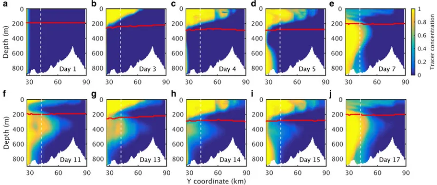
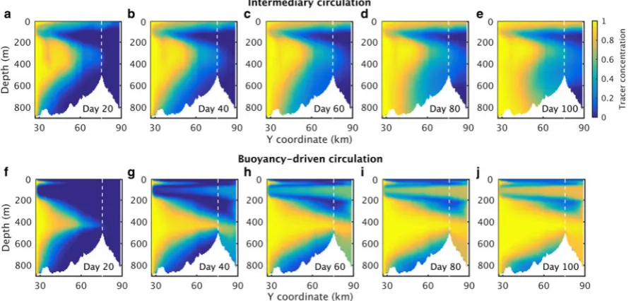
Fig. 4. Fjord centreline sections showing the movement of water from the shelf (represented by a tracer concentration of 1, yellow) into the fjord over the course of two consecutive wind events using the standard shelf forcing (i.e. with the PW/AW interface on the shelf depressed by 100 m for two periods of 2 d, centred on days 4 and 14). Theσϴ=27.3 kg m−3isopycnal is shown by the red line. The velocity profiles across

value of 1 as it is exported from the fjord, which is equivalent to assuming there is no return flow of exported fjord waters. Return flow to fjords and estuaries has been estimated to lie in the range of 0–50% (e.g. Luketina, 1998; Gillibrand, 2001), and is highly dependent on the strength of shelf cur-rents and the frequency of the oscillations in the fjord circu-lation. Any return flow will reduce the efficiency of fjord flushing; because we assume no return flow, our experiments should therefore be considered as upper bounds for the likely rate of fjord renewal for the simulated modes of circulation when considered in isolation.

4. RESULTS

4.1. Intermediary circulation

We find that current velocities in KF are commensurate with those observed during large wind events at SF when we force the model withΔhi=100 m, which is at the upper end of the

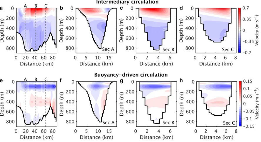
range of isopycnal fluctuations observed at that fjord (Jackson and others,2014), andt=2 d (Figs 3and4). This is hence-forth referred to as thestandard shelf forcing. The resulting exchange can be divided into two phases. In the first, the enforced depression of the PW/AW interface on the shelf is rapidly transmitted up-fjord (Figs 4a–c), facilitated by an inflow of water in the PW layer and outflow of water in the AW layer (Figs 3,4b,c). In the second phase (after the face has been held in its depressed position for 2 d) the inter-face on the shelf begins to rise back towards its original depth, causing an outflow of water in the PW layer and an inflow of water from the shelf in the AW layer (Figs 3,4d,e). Under this forcing, the maximum velocity in the PW layer at section B peaks at∼0.7 m s−1(Fig. 3a), or∼0.3 m s−1if averaged across the width and depth of the PW layer at this section (Fig. 3b). During the periods of peak flow (Figs 5a–d), circulation within the fjord is predominantly 2-D,

though greater across-fjord variability occurs as the trough broadens outside of the fjord mouth (Fig. 5b). The transport of water up- and down-fjord is approximately equal (Fig. 3c) and so the relative velocities in the two layers are determined by their thicknesses: the transport in the PW layer must be accommodated in a thinner layer, and so vel-ocities are greater than those in the AW layer.

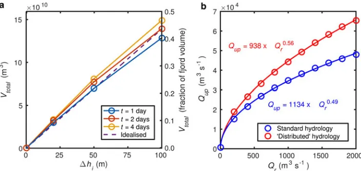
During each phase, a volume of water from the shelf is exchanged with an equal volume of water from the fjord. If the fjord is able to fully adjust to the depression of the shelf stratification, the volume exchanged in each phase should be approximately equal toΔhiA, whereA is the plan area

of the fjord (e.g. Arneborg,2004). During the first phase, a volumeVIof AW from within the fjord is replaced with PW

from the shelf; in the second phase, a volume VII of PW

from within the fjord is replaced with AW from the shelf. The total volume exchange,Vtotal, is equal toVI+VII, and

can be calculated as the integrated up-fjord volume transport across the fjord mouth over the course of the two phases. Vtotalshould be approximately equal to 2ΔhiA, and there is

a good agreement between this idealised scenario and that predicted by the model simulations (Fig. 6a).

Vtotalmay be equal to a significant proportion of the fjord

volume: for the standard shelf forcing,Vtotalis equal to∼40%

of the total fjord volume (Fig. 6a). However, because a frac-tion of the PW imported during the first phase (Figs 4b,c) is re-exported during the second phase (Figs 4d, e), Vtotal

over-estimates the increase in the shelf water content of the fjord over the course of a wind event. Based on the passive tracer concentration, the first instance of the standard shelf forcing results in a new fjord composition that is only

∼28% imported shelf water and∼72% original fjord water. Similarly, much of the AW imported during the latter phase of the first wind event (Figs 4d,e) is then exported from the fjord during the first phase of the following wind event (Figs 4f, h); for a second wind event 10 d later, the net

increase in the shelf water content of the fjord is only∼9% (Fig. 4j). This recycling of water between the fjord and shelf strongly influences the rate at which the intermediary circu-lation is able to drive fjord renewal, and is discussed further in Section 5.3.

4.2. Buoyancy-driven circulation

An example of the modelled summer buoyancy-driven circu-lation is shown inFigures 5e–h, which shows the circulation resulting from the mean July runoff input (900 m3s−1) to the fjord (henceforth referred to as the summer runoff forcing). The strongest currents (∼0.1 m s−1) flow down-fjord immedi-ately above the PW/AW interface (∼50–150 m depth), and result from the intrusion of glacially modified water (GMW, a mixture of runoff, ice melt and fjord water) from many of the larger runoff-driven plumes that reach neutral buoyancy at this steep density gradient. There are also weaker down-fjord currents at the surface (resulting from the shallower input of runoff at smaller glaciers) and at ∼200–300 m depth (resulting from the smaller runoff inputs from deep gla-ciers that lack the buoyancy to reach the PW/AW interface). Below these layers (and to a lesser extent between the surface and interface (e.g.Figs 5g,h)), flow is directed up-fjord, re-placing water entrained into the GMW. There is some across-fjord heterogeneity in the velocity structure, with cur-rents deflected to the right by the Coriolis effect, most notably where the fjord widens as it joins the shelf (Fig. 5f).

We find that the relationship between subglacial melt-water runoff, Qr, and the up-fjord volume transport across

the fjord mouth,Qup, takes the formQup=aQrb, whereais ∼1000 and the exponentbhas a value of∼1/2 (Fig. 6b). It has been demonstrated that for a rectangular, flat-bottomed fjord,Qupis greater for a given Qr if this runoff is divided

evenly between a larger number of channels (Carroll and others, 2015). To test whether our chosen distribution of runoff inputs (Section 3.4.2) is an important control on the strength ofQupin our simulations of KF, we experimented

with an alternative configuration in which the runoff from each glacier was distributed evenly between channels

located at 500 m intervals along their calving fronts. We find that the volume transport generated by this scenario is up to∼35% greater (Fig. 6b) than for the standard hydrologic-al configuration (in which 90% of runoff is input from a single channel at each glacier). The form of the relationship betweenQrandQupis however similar for the two

hydro-logical configurations, with Qup proportional to Qr to the

power of ∼1/2, suggesting the relative variability in the strength of the buoyancy-driven circulation may not be sen-sitive to the near-terminus hydrology. Nevertheless, it is likely that the distribution of subglacial channels remains a critical control on other features of ice/ocean interaction, particularly the strength and distribution of submarine melting (Fried and others, 2015; Slater and others, 2015), and, as such, improving our knowledge of marine-terminat-ing glacier hydrology remains a key area for research.

5. DISCUSSION

5.1. Comparison of modelled fjord circulation with observations

Observations from KF and SF have revealed two prominent circulation regimes in these large East Greenland fjords. In the first regime, recorded by continuous over-winter moor-ings, circulation is dominated by fast (up to∼0.8 m s−1), peri-odically reversing currents with a predominantly two-layer structure (Jackson and others,2014). In the second, captured during a survey in late summer, circulation is characterised by slightly slower currents (up to ∼0.4 m s−1) and a more complex structure, with the strongest down-fjord currents found at ∼100–300 m below the surface (Sutherland and others,2014).

The two modes of circulation simulated in this paper agree well with these two observed regimes. The simulated inter-mediary circulation agrees well with the observed winter cir-culation (Figs 3,5a–d), demonstrating the influence of shelf conditions on the fjord at a time of year when coastal storms are at their strongest and most frequent, and runoff is at its annual minimum (Jackson and others, 2014). The

Fig. 6. (a) Volume of water exchanged between the shelf and fjord due to intermediary circulation over a 10 d window (Vtotal), shown as a function ofΔhiandt. Note thatVtotalis not equal to the volume of new shelf water in the fjord at the end of the 10 d period, as a proportion of the water imported during the depression of the PW/AW interface is re-exported during the subsequent raising of this interface (Section 4.1). The dashed‘idealised’line showsVtotalcalculated as 2ΔhiA, whereAis the plan area of the fjord. (b) Up-fjord volume transport,Qup, across the fjord mouth as a function of runoff inputQr. For the standard hydrology (blue), runoff is input as described in Section 3.4.2. In the

simulated buoyancy-driven circulation more closely resem-bles the observed summer circulation, particularly with respect to the export of waters in the region of the PW/AW interface (Figs 5e–h). While this similarity alone is insufficient to rule out the possibility that other forcings may influence the observed summer circulation, it is intuitive that buoy-ancy-driven circulation is of greatest importance at a time of year when runoff of fresh water is highest and storms are less frequent. Further support for this hypothesis comes from Inall and others (2014), who found the temperature and salinity structure of KF during late summer to be com-mensurate with a steady, layered exchange flow, driven by the input of glacial runoff at depth.

5.2. Mixing in glacial plumes

As described in Section 4.2, we find that for the buoyancy-driven circulation scenarios, the up-fjord volume transport Qup is proportional to Qr∼1/2. Qup represents the transport

of water required to replace the fjord waters entrained into the GMW and subsequently exported from the fjord. Over the range of Qr used in the experiments (0–2000 m3s−1),

Qup is one or two orders of magnitude >Qr (Fig. 6b).

Because water is input from multiple glaciers around the fjord, it is difficult to partition this entrainment between that occurring in the runoff-driven plumes (as parameterised using plume theory), and mixing throughout the remainder of the fjord. To examine this more closely, we therefore briefly consider a simpler set up in which only runoff from KG (which in the standard set up accounts for∼55% of the total runoff input to KF) is included. In this scenario, 87% of entrainment occurs in the innermost 5 km of the fjord (up-fjord of section D inFig. 1a), while 13% occurs through-out the remainder of the fjord (Table 1). This suggests that the circulation is driven primarily by processes occurring in the plume region adjacent to the glaciers. Care is however required in comparing the rate of entrainment by the vertical plume with that occurring throughout the fjord, as these two processes depend on different model parameterisations: the former is parameterised through buoyant plume theory (Cowton and others,2015) while the latter is dependent on subgrid mixing schemes in MITgcm. Furthermore, the omis-sion of additional mixing processes including tides and along-fjord winds (e.g. Farmer and Freeland, 1983) may cause mixing in the fjord to be underestimated, in which caseQupshould increase more rapidly between section D

and the fjord mouth (Fig. 1a). Nevertheless, a robust finding is that even if mixing throughout the remainder of the fjord is not considered, entrainment into the plumes immediately

around the calving front is sufficient to drive a significant ex-change between the fjord and shelf during the summer months when there is a substantial runoff input.

5.3. Renewal of fjord waters

From a glaciological perspective, the most important func-tion of the fjord circulafunc-tion is its role in controlling water properties at the calving fronts of marine-terminating gla-ciers, the largest of which are often found at the heads of fjords. We examine this function by quantifying the rate at which waters within the fjord are renewed by waters from the shelf. This determines the rate at which oceanic heat is supplied to the fjord, and provides an indication of the time-scales over which glaciers draining into the fjord may experi-ence the variations in ocean temperature occurring on the shelf beyond the fjord mouth.

The timescale of fjord renewal can be expressed through the turnover time TE (Prandle, 1984; Gillibrand, 2001),

which describes the time taken for fjord/shelf exchange to dilute the original contents of the fjord by a factor 1–e−1 (i.e. until the fjord contains 37% of the original fjord water and 63% water imported from the shelf). We calculate TE

for the modelled circulation in KF by tracking the movement of the passive tracer into the fjord over time (Figs 7and8). In the intermediary circulation scenarios, TE will depend not

only on the magnitude of the applied shelf forcing, but also on the periodicitypat which the perturbation of the interface is applied. Jackson and others (2014) report that in SF the pulses associated with intermediary circulation occur on syn-optic timescales, with a dominant periodicity of 4–10 d. Similarly, Harden and others (2011) found the average peri-odicity of winter storms off East Greenland to vary between

∼5 and 13 d over the period 1989–2008. Our standard shelf forcing requires a minimum of 6 d (2 d each with the interface on the shelf in its unperturbed and depressed state, and two transition days; i.e. day 1.5–7.5 in Fig. 3a), and so we test the sensitivity of TE to p over the range of

6–14 d (Figs 8a,b).

To place these results into context, we compare them with a simple‘slab’model of intermediary circulation (Arneborg, 2004). Based on three decades of observations from Gullmar Fjord, Sweden, Arneborg (2004) proposed that the turnover time of a fjord as a result of intermediary circulation can be approximated as

TE¼p

hs

σðhiÞ ð1Þ

whereσ(hi) is the standard deviation of the upper layer

thick-ness (in our case synonymous with the standard deviation of the PW/AW interface depth) andhsis the sill depth (500 m).

The solution of the slab model is in reasonable agreement with the fjord simulations, albeit with a greater sensitivity of TEtop (Fig. 8b). This discrepancy may in part be because

we depresshifor a fixed period of 2 d (Fig. 3a), rather than

allowing the duration of the perturbation to scale withp, as well as likely reflecting the simplified nature of the slab model. A notable feature of the fjord simulations, in contrast to the slab model, is that there is no further reduction inTE

when p is reduced below 8 d, reflecting the trade-off between the increased frequency of the intermediary circula-tion events and the reduced exchange that can take place during each event. We are therefore able to place

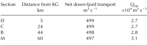
Table 1. Net down-fjord volume transport, and up-fjord volume transportQupacross sections D, C, B and M inFig. 1a, for a subgla-cial discharge of 500 m3s−1from KG only. The slight down-fjord decline in net transport occurs because the boundary flux does not perfectly balance the runoff input

Section Distance from KG Net down-fjord transport Qup

km m3s−1 ×104m3s−1

D 5 499 2.7

C 24 499 2.7

B 44 498 2.8

approximate bounds on the value of TE for the standard

shelf forcing–based on a high frequency of winter storms (p≤8 d), TE∼90 d, while for a low frequency of winter

storms (p=13 d),TE∼130 d.

A key difference between KF and Gullmar Fjord (and many other smaller, mid-latitude fjords) is the depth of the sill. The ratio σ(hi)/hs in Eqn (1) represents the relative

volume changes associated with the fluctuations in the inter-face depth. At Gullmar Fjord, Arneborg (2004) reported σ

(hi)=6.6 m and hs=43 m, giving a ratio of 0.15. For the

standard shelf forcing at KF,σ(hi)=42 m (forp=10 d) and

hs=500 m, giving a ratio of 0.084. This means that for a

given value ofp, the slab model predicts that the turnover time at KF will be nearly a factor of two greater than that for Gullmar Fjord, despite the much larger forcing at KF.

While the intermediary circulation in KF may therefore be capable of generating a vigorous exchange between the fjord and shelf, these findings suggest that the great depth of the fjord reduces the efficacy of this process as a mechan-ism of fjord renewal. This point is supported by the findings of Gladish and others (2015) who used a 2-D numerical model to examine the circulation of Jakobshavn Isfjord in West Greenland; despite removing the sill to allow free communi-cation between the fjord and shelf, they found that vigorous intermediary circulation was not effective at renewing this

∼800 m deep fjord compared with circulation resulting from submarine ice melt and, more notably, runoff input.

Direct comparison of the two modes of circulation is diffi-cult because the oscillatory nature of the intermediary circu-lation contrasts with the steady buoyancy-driven circucircu-lation.

Fig. 7. Fjord centreline sections showing the movement of water from the shelf (represented by a tracer concentration of 1, yellow) into the fjord over the course of 100 d for the standard shelf forcing withp=10 d (a–e) and the summer runoff forcing (f–j) (see alsoFig. 8). The scale on the horizontal axis refers to theY-coordinates inFigure 1a. The fjord mouth section (M) forms the left hand limit of the plots, while the upper sill section (S) is marked by the dashed line.

The total volume exchange,Vtotal, associated with each

in-stance of the standard shelf forcing is ∼1.4 × 1011_m3

(Fig. 6a). Over an equivalent 10 d period, the cumulative up-fjord transport of water (i.e. time-integratedQup) due to

the summer runoff forcing is only ∼0.3 × 1011m3. The turnover times (calculated using the passive tracer) for the intermediary circulation and summer buoyancy-driven cir-culation scenarios are however much more similar, being 105 d for the summer buoyancy-driven circulation and

∼90–130 d (forp=6–13 d) for the intermediary circulation (Fig. 8). Furthermore, and critically for ocean/ice interaction, the modelled summer buoyancy-driven circulation is much more effective at transporting water to the fjord head relative to the intermediary circulation. In the summer runoff forcing scenario, water from outside the fjord mouth reaches the fjord head within 40 d (Fig. 7g). After 100 d, this buoyancy-driven circulation has replaced∼65% of the waters within the innermost 13 km of the fjord (i.e. the branch containing KG) with shelf water, compared with <30% for the inter-mediary circulation scenarios (Figs 7,8).

These differences in the efficiency of fjord renewal between the intermediary and buoyancy-driven circulation occur for two main reasons. Firstly, the buoyancy-driven cir-culation is steady over time during the melt season, with a persistent up-fjord current at depth (Figs 3b,c,5e–h, 7f–j). This contrasts with the intermediary circulation, where the same water may be exchanged repeatedly across the fjord mouth as the currents reverse (Figs 3,4). Secondly, the buoy-ancy-driven circulation is driven by the inputs of freshwater at the head of the fjords, meaning the circulation is effective at drawing water all the way to the glacier termini. The inter-mediary circulation, on the other hand, is most effective at exchanging water in the outer part of the fjord, and much less effective at driving shelf water up to the fjord heads. It is also important to note that for the summer runoff forcing, the proportion of shelf water in the inner fjord becomes greater than the average throughout the fjord after ∼70 d (Fig. 8a). This occurs because the plumes near to the KG ter-minus generate significant vertical mixing, redistributing shelf waters through a greater part of the water column (Fig. 7h).

The summer runoff forcing is based on the input to the fjord of∼900 m3s−1of runoff from surface melting of the ice sheet, but this will be negligible during the∼7 non-summer months. It is however likely that some year-round input of runoff con-tinues due to basal melting of the ice sheet through geothermal and frictional heating (Christoffersen and others,2012). This flux is hard to quantify, but a likely indication of the approxi-mate magnitude comes from Store Glacier, a large marine-ter-minating outlet glacier in West Greenland, where Chauché (2016) used hydrographic data from the fjord to estimate an average winter runoff of 36 ± 22 m3s−1. Taking 50 m3s−1as a generous estimate for winter runoff from KG and scaling runoff input from the other glaciers accordingly (see Section 3.4.2) gives a total winter runoff forcing of∼90 m3s−1, an order of magnitude smaller than the summer runoff forcing. In this scenario,TE (300 d) far exceeds that for the summer

buoyancy-driven circulation and the intermediary circulation scenarios (∼100 d) (Fig. 8). In the inner fjord, however, there is a similar rate of increase in the shelf water concentration between the winter runoff scenario and the intermediary circu-lation scenarios, with this concentration reaching∼60% after 300 d (Fig. 8). Alternatively, a conservative estimate of the winter buoyancy-driven circulation can be obtained by

specifying zero runoff such that circulation is driven only by submarine melting (although these results should be treated cautiously as melt-driven convection at the calving fronts will be poorly represented at the coarse model resolution and melting of icebergs and ice mélange is not considered). In this no runoff forcing scenario, the buoyancy-driven circu-lation is much weaker such that only ∼35% of the fjord volume (and<10% of the upper fjord) is replaced with shelf waters over the 300 d of the model run (Fig. 8c). These experi-ments indicate that while we expect buoyancy-driven circula-tion to dominate the transport of shelf waters to the inner fjord during the summer months, outside of the melt season the dominant mode of transport is less clear. If there is a sufficient input of runoff from basal melting, then buoyancy-driven cir-culation may remain significant year-round; if not, then inter-mediary circulation will likely dominate in winter. In either case, the weak currents associated with the winter buoy-ancy-driven circulation will likely be obscured by the inter-mediary circulation, consistent with the finding by Jackson and others (2014) that buoyancy-driven circulation is not visible in winter velocity observations obtained at SF.

It should also be noted that while we find the simulated intermediary circulation is comparatively limited in its ability to advect new shelf waters to the fjord head, we do not exclude the possibility that alternative shelf-driven exchanges could be more effective at renewing waters along the length of the fjord. In our simulations, we have focused on the intermediary circulation driven by along-shore shelf winds, given the proposed importance of this mechanism for fjord renewal (e.g. Straneo and Cenedese, 2015). However, it is possible, for example, that the arrival of a new water mass on the shelf, or the steering of ocean cur-rents along the cross-shelf troughs leading to KF and SF (e.g. Christoffersen and others,2011; Magaldi and others,2011), could drive an exchange that is more effective at advecting shelf water to the fjord head. Assessment of these mechan-isms would require observations from and/or modelling of a much larger region of the shelf surrounding the fjord, and as such lies beyond the scope of this paper.

5.4. Up-fjord heat transport due to buoyancy-driven circulation

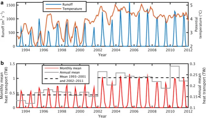
It has been hypothesised that the retreat of many of Greenland’s marine-terminating glaciers has been driven by the warming of ocean waters off Greenland since the mid-1990s (Straneo and Heimbach,2013). Our results indi-cate that buoyancy-driven circulation, resulting from the input of glacial runoff, provides an effective mechanism for the transport of this oceanic heat from the shelf to the glaciers at sub-seasonal timescales. Through this mechanism the heat transport will increase not only with ocean temperature but also with atmospheric temperature, which controls the input of meltwater runoff to the fjord. To examine the re-sponse of heat transport to climatic variability, we calculated the heat transportHdue to the buoyancy-driven mode of cir-culation into KF at monthly intervals over a 19 year period from 1993 to 2011. This is calculated as

H¼cpρ0Qupðθshelf θfÞ ð2Þ

wherecpis the specific heat capacity of sea water (3980 J

kg−1K−1),ρ0is a reference density (1027 kg m−3) andθshelf

mouth (°C).θfis the depth-averaged freezing point (−2.17°C,

based on the initial salinity stratification;Fig. 1c); we use this value as the reference temperature because our primary interest lies in the variability in the heat available for melting at the calving front.

To obtain a time series ofθshelf, we utilise the GLORYS2V3

1/4° ocean reanalysis product (Ferry and others,2012).θshelf

is taken as the depth-averaged temperature of these reanaly-sis data between 200 and 500 m depth (Fig. 9a), shown in the modelling experiments to represent the main depth-range of up-fjord flow (Figs 7f–j), in the cell where KF joins the shelf (the fjord itself is not resolved in the reanalysis). Comparison with available hydrographic surveys at the fjord mouth (e.g. Inall and others, 2014; Sutherland and others,2014) suggests the reanalysis AW temperature is typ-ically∼1°C warmer than the observations, which may reflect across-shelf cooling of subsurface waters not captured by the reanalysis (e.g. Christoffersen and others, 2011). This bias will act to slightly reduce the apparent relative variability in

θshelf–θf, meaning the calculated relative change inHmay

be slightly underestimated. For example, an increase in

θshelffrom 2 to 3°C would cause H to increase by∼25%,

whereas an increase inθshelffrom 3 to 4°C would causeH

to increase by only∼20%.

Qup is calculated according to the values given for the

‘standard hydrology’curve inFigure 6b, using the modelled catchment-wide runoff input to KF over this period (Fig. 9a). Given the uncertainty with respect to the basal melt rate, and how this may vary over time (e.g. due to glacier acceler-ation), we do not prescribe a contribution to runoff from basal melting. The results of this section therefore reflect only the buoyancy-driven circulation in response to the runoff of meltwater from melting of the ice-sheet surface.

We emphasise that we seek here to estimate only the up-fjord transport of oceanic heat due to buoyancy-driven circulation, and not the difference between the up- and down-fjord heat transport, which would require accurate quantification of the use of this heat in melting of the

glacier calving fronts or icebergs/ice mélange. In this ap-proach we differ from previous numerical modelling studies that have sought to quantify the submarine melt rate resulting from variation in runoff and fjord water temperature (e.g. Sciascia and others,2013; Xu and others,2013; Slater and others,2015). We do this for two reasons. Firstly, mod-elled submarine melt rates are strongly dependent on turbu-lent transfer coefficients within the model (Holland and Jenkins, 1999) and the prescribed distribution of runoff at the grounding line (Slater and others,2015), both of which are poorly constrained by observations. Secondly, it remains unclear whether (and if so how) submarine melting influences the stability of fast flowing outlet glaciers such as KG, where the thickness and rigidity of ice mélange and the seasonal duration of land-fast sea ice may also be import-ant controls on calving rate (e.g. Amundson and others, 2010; Christoffersen and others, 2012; Nick and others, 2013). By focusing simply on the heat available in the prox-imity of KG’s terminus, we avoid prescribing a specific mech-anism linking ocean temperature to glacier stability, instead recognising that an increase in oceanic heat availability may lead to glacier retreat through one or a combination of mechanisms.

The modelled up-fjord heat transport due to buoyancy-driven circulation is shown in Figure 9b. The sub-linearity of the relationship between runoff and volume transport reduces the interannual variability in heat transport relative to runoff. Nevertheless, both runoff and ocean temperature increased markedly in the early 2000s, resulting in a∼50% increase in the mean value of H between the periods 1993–2001 and 2002–11 (Fig. 9). The timing of this increase agrees closely with the acceleration of mass loss from KG, with the glacier thinning between 2003 and 2004 then undergoing a phase of rapid retreat and thinning through 2004/05 (Luckman and others, 2006; Howat and others, 2007), suggesting the possible role of oceanic heat in trigger-ing retreat. While our modelltrigger-ing work has focused on KF and KG, this finding is likely to be equally applicable to many

glaciers along Greenland’s southeast coast, which under-went a synchronous thinning and retreat in response to re-gional oceanic and atmospheric warming at this time (e.g. Seale and others,2011).

6. CONCLUSIONS

In this paper we have used a 3-D numerical model of KF, East Greenland, to examine controls on fjord/shelf exchange and the transport of oceanic heat to marine-terminating glaciers. We have focussed on two key mechanisms: intermediary cir-culation forced by fluctuations in the depth of isopycnals on the shelf (due to the passage of coastal storms), and buoy-ancy-driven circulation forced by the input of glacial meltwater.

Comparison between the modelled circulation and field observations (Jackson and others, 2014; Sutherland and others, 2014) demonstrates that the model captures these key mechanisms of circulation in the fjord. The intermediary circulation takes the form of a fast (up to∼0.7 m s−1), period-ically reversing, two-layer exchange. The buoyancy-driven circulation (forced by the input of runoff at depth from mul-tiple glaciers) forms a more complex multi-celled circulation, with the strongest outflow (∼0.1 m s−1) occurring around the PW/AW interface. We find that the rate of buoyancy-driven exchange between the fjord and shelf (controlled principally by mixing in plumes at the glacier termini) scales with runoff to the power of ∼1/2, with the exchange rate one to two orders of magnitude greater than the initial runoff input.

Over short timescales, and in keeping with observations, we find that exchanges associated with intermediary circula-tion can exceed those due to buoyancy-driven circulacircula-tion. During a 10 d period associated with the passage of a coastal storm, the modelled intermediary circulation can ex-change up to∼25% of the fjord volume with shelf waters. In comparison, at its strongest in midsummer, the buoyancy-driven circulation replaces∼10% of the fjord volume with shelf waters over an equivalent 10 d period. The rapid ex-change associated with the intermediary circulation means that water properties in the outer reaches of the fjord are able to track changes occurring on the shelf over timescales of only a few days.

In spite of this rapid exchange in the outer fjord, we find that intermediary circulation is not effective at transporting waters from the shelf to the glacier termini. This is because intermediary circulation is periodically reversing, meaning imported shelf waters tend to be subsequently re-exported back to the shelf rather than transported further up-fjord. In contrast, the temporal consistency of buoyancy-driven circu-lation means that it is much more effective at transporting subsurface waters from the shelf to the glaciers at the fjord head. This is illustrated by calculating the turnover time for the innermost 13 km of the fjord:∼100 d for the buoyancy-driven circulation (under summer conditions), compared with>250 d for the most intense intermediary circulation scenarios.

During the summer months, when meltwater runoff is greatest and coastal storms are weaker and less frequent, we therefore expect buoyancy-driven circulation to domin-ate the up-fjord transport of oceanic heat. Outside of the melt season, runoff from ice-sheet basal melting may be suf-ficient to allow buoyancy-driven circulation to continue to play a significant, albeit reduced, role; if not, intermediary

circulation will be the dominant mode of fjord circulation during the winter months.

Because the strength of the buoyancy-driven circulation increases with runoff, a greater quantity of oceanic heat will be advected to the glaciers during longer and warmer summers. We estimate that mean heat transport to KG due to buoyancy-driven circulation increased ∼50% between the periods 1993–2001 and 2002–11, with annual up-fjord heat transport in 2004/05 double that of the cooler years of the early to mid-1990s. This increased heat availability has the potential to influence glacier stability by increasing sub-marine melting at the calving front, weakening the ice mélange or decreasing the duration of seasonal sea-ice cover, all of which may have contributed to the retreat of KG (and many other marine-terminating glaciers in southeast Greenland) in the early years of the 21st century.

SUPPLEMENTARY MATERIAL

The supplementary material for this article can be found at http://dx.doi.org/10.1017/jog.2016.117

ACKNOWLEDGEMENTS

The authors would like to thank: Julian Dowdeswell and Karen Heywood for the provision of bathymetry and tem-perature and salinity data respectively (collected during James Clark Ross Cruise JR106b with the support of NERC’s Autosub Under Ice Thematic Programme and NERC grant NER/T/S/2000/0099); the GLORYS project for providing ocean reanalysis data (GLORYS is jointly conducted by MERCATOR OCEAN, CORIOLIS and CNRS/INSU); CReSIS for the provision of basal topography for KG (generated with support from NSF grant ANT-0424589 and NASA grant NNX10AT68G); Philippe Huybrechts for his contribu-tion to the runoff model used in this paper; and two anonym-ous referees whose constructive and insightful reviews made a valuable contribution to the paper. This work was funded by NERC grant NE/K014609/1 to Peter Nienow and Andrew Sole and a NERC studentship to Donald Slater. Edward Hanna and David Wilton acknowledge support from NERC grant NE/H023402/1. Please contact the corre-sponding author attom.cowton@st-andrews.ac.ukto obtain the data or numerical model described in this paper.

REFERENCES

Adcroft A, Hill C, Campin J, Marshall J and Heimbach P (2004) Overview of the formulation and numerics of the MIT GCM. In

Proceedings of the ECMWF Seminar Series on Numerical Methods, Recent Developments in Numerical Methods for Atmosphere and Ocean Modelling, 139–149.

Amundson J and 5 others (2010) Ice melange dynamics and impli-cations for terminus stability, Jakobshavn Isbrae Greenland.

J. Geophys. Res.-Earth Surf., 115, F01005 (doi: 10.1029/ 2009jf001405)

Arneborg L (2004) Turnover times for the water above sill level in Gullmar Fjord. Cont. Shelf Res., 24(4–5), 443–460 (doi: 10.1016/j.csr.2003.12.005)

Chauché N (2016)Glacier-Ocean interaction at Store Glacier (West Greenland). Doctor of Philosophy, Department of Geography and Earth Science, Aberystwyth University.

Chauché N and 8 others (2014) Ice-ocean interaction and calving front morphology at two west Greenland tidewater outlet glaciers.

Cryosphere,8(4), 1457–1468 (doi: 10.5194/tc-8-1457-2014) Christoffersen P and 7 others (2011) Warming of waters in an East

Greenland fjord prior to glacier retreat: mechanisms and connec-tion to large-scale atmospheric condiconnec-tions.Cryosphere,5, 701–

714 (doi: 10.5194/tc-5-701-2011)

Christoffersen P, O’Leary M, Van Angelen J and van den Broeke M (2012) Partitioning effects from ocean and atmosphere on the calving stability of Kangerdlugssuaq Glacier, East Greenland.

Ann. Glaciol.53(60), 249–256 (doi: 10.3189/2012AoG60A087) Cowton T, Slater D, Sole A, Goldberg D and Nienow P (2015) Modeling the impact of glacial runoff on fjord circulation and submarine melt rate using a new subgrid-scale parameterization for glacial plumes. J. Geophys. Res., 120, 796–812 (doi: 10.1002/2014JC010324)

Dowdeswell J (2004) Cruise report - JR106b. RSS James Clark Ross. NERC Autosub Under Ice thematic programme, Kangerdlugssuaq Fjord and shelf, east Greenland.

Enderlin E and 5 others (2014) An improved mass budget for the Greenland ice sheet.Geophys. Res. Lett., 41(3), 866–872 (doi: 10.1002/2013gl059010)

Farmer D and Freeland H (1983) The physical oceanography of fjords. Prog. Oceanogr., 12(2), 147–219 (doi: 10.1016/0079-6611(83)90004-6)

Ferry N and 6 others (2012) Scientific Validation Report (ScVR) for Reprocessed Analysis and Reanalysis. MyOcean project report, MYO-WP04-ScCV-rea-MERCATOR-V1.0.

Fried M and 8 others (2015) Distributed subglacial discharge drives significant submarine melt at a Greenland tidewater glacier.

Geophys. Res. Lett., 42(21), 1944–8007 (doi: 10.1002/ 2015GL065806)

Garvine R (1995) A dynamical system for classifying buoyant coastal discharges.Cont. Shelf Res.,15(13), 1585–1596 (doi: 10.1016/ 0278-4343(94)00065-u)

Gillibrand P (2001) Calculating exchange times in a Scottish fjord using a two-dimensional, laterally-integrated numerical model.

Estuar. Coast. Shelf Sci. 53(4), 437–449 (doi: 10.1006/ ecss.1999.0624)

Gladish C, Holland D, Rosing-Asvid A, Behrens J and Boje J (2015) Oceanic boundary conditions for Jakobshavn glacier. Part I: vari-ability and renewal of ilulissat icefjord waters, 2001–14.J. Phys. Oceanogr.,45(1), 3–32 (doi: 10.1175/jpo-d-14-0044.1) Griffies S and Hallberg R (2000) Biharmonic friction with a

Smagorinsky-like viscosity for use in large-scale eddy-permitting ocean models. Mon. Weather Rev., 128(8), 2935–2946 (doi: 10.1175/1520-0493(2000)128<2935:bfwasl>2.0.co;2) Hanna E and 5 others (2009) Hydrologic response of the Greenland

ice sheet: the role of oceanographic warming.Hydrol. Process., 23(1), 7–30 (doi: 10.1002/hyp.7090)

Hanna E and 12 others (2011) Greenland Ice Sheet surface mass balance 1870 to 2010 based on Twentieth Century Reanalysis, and links with global climate forcing.J. Geophys. Res.: Atmos. (1984–2012),116(D24), D24121 (doi: 10.1029/2011JD016387) Harden B, Renfrew I and Petersen G (2011) A climatology of

winter-time barrier winds off Southeast Greenland. J. Clim., 24(17), 4701–4717 (doi: 10.1175/2011jcli4113.1)

Holland D and Jenkins A (1999) Modeling thermodynamic ice-ocean interactions at the base of an ice shelf. J. Phys. Oceanogr., 29(8), 1787–1800 (doi: 10.1175/1520-0485(1999) 029<1787:mtioia>2.0.co;2)

Howat I, Joughin I and Scambos T (2007) Rapid changes in ice dis-charge from Greenland outlet glaciers. Science, 315(5818), 1559–1561 (doi: 10.1126/science.1138478)

Inall M and 6 others (2014) Oceanic heat delivery via Kangerdlugssuaq Fjord to the south-east Greenland ice sheet.J.

Geophys. Res.: Oceans, 119(2), 631–645 (doi: 10.1002/ 2013JC009295)

Jackson R, Straneo F and Sutherland D (2014) Externally forced fluc-tuations in ocean temperature at Greenland glaciers in non-summer months. Nat. Geosci., 7(7), 503–508 (doi: 10.1038/ ngeo2186)

Janssens I and Huybrechts P (2000) The treatment of meltwater retention in mass-balance parameterizations of the Greenland ice sheet. Ann. Glaciol. 31, 133–140 (doi: 10.3189/ 172756400781819941)

Jenkins A (2011) Convection-driven melting near the grounding lines of ice shelves and tidewater glaciers.J. Phys. Oceanogr., 41(12), 2279–2294 (doi: 10.1175/jpo-d-11-03.1)

Klinck J, Obrien J and Svendsen H (1981) A simple model of fjord and coastal circulation interaction.J. Phys. Oceanogr., 11(12), 1612–1626 (doi: 10.1175/1520-0485(1981)011<1612:asmofa> 2.0.co;2)

Leuschen C and Allen C (2013)IceBridge MCoRDS L3 Gridded Ice Thickness, Surface and Bottom, Version 2, Kangerdlugssuaq 2008–2012 Composite. NASA DAAC at the National Snow and Ice Data Center, Boulder, Colorado, USA.

Losch M (2008) Modeling ice shelf cavities in a z coordinate ocean general circulation model.J. Geophys. Res.-Oceans, 113(C8), C08043 (doi: 10.1029/2007jc004368)

Luckman A, Murray T, de Lange R and Hanna E (2006) Rapid and synchronous ice-dynamic changes in East Greenland.

Geophys. Res. Lett.,33(3), L03503 (doi: 10.1059/2005gl025048) Luketina D (1998) Simple tidal prism models revisited.Estuar. Coast.

Shelf Sci.,46(1), 77–84 (doi: 10.1006/ecss.1997.0235)

Magaldi M, Haine T and Pickart R (2011) On the nature and variabil-ity of the East Greenland spill jet: a case study in summer 2003.J. Phys. Oceanogr., 41(12), 2307–2327 (doi: 10.1175/jpo-d-10-05004.1)

Morton B, Taylor G and Taylor J (1956) Turbulent gravitational con-vection from maintained and instantaneous sources.

Proc. R. Soc. London Ser. A-Math. Phys. Sci.,234(1196), 1–23 (doi: WOS:A1956WU30300001)

Nick F and 7 others (2013) Future sea-level rise from Greenland’s main outlet glaciers in a warming climate.Nature, 497(7448), 235–238 (doi: 10.1038/nature12068)

Prandle D (1984) A modelling study of the mixing of Cs-137 in the seas of the European continental shelf.Philos. Trans. R. Soc. A-Math. Phys. Eng. Sci., 310(1513), 407–436 (doi: 10.1098/ rsta.1984.0002)

Rignot E and Kanagaratnam P (2006) Changes in the velocity struc-ture of the Greenland ice sheet.Science,311(5763), 986–990 (doi: 10.1126/science.1121381)

Rignot E, Fenty I, Menemenlis D and Xu Y (2012) Spreading of warm ocean waters around Greenland as a possible cause for glacier acceleration. Ann. Glaciol., 53(60), 257–266 (doi: 10.3189/ 2012AoG60A136)

Rignot E, Fenty I, Xu Y, Cai C and Kemp C (2015) Undercutting of marine-terminating glaciers in West Greenland.Geophys. Res. Lett.,42(14), 5909–5917 (doi: 10.1002/2015gl064236) Sciascia R, Straneo F, Cenedese C and Heimbach P (2013) Seasonal

variability of submarine melt rate and circulation in an East Greenland fjord.J. Geophys. Res.-Oceans,118(5), 2492–2506 (doi: 10.1002/jgrc.20142)

Sciascia R, Cenedese C, Nicoli D, Heimbach P and Straneo F (2014) Impact of periodic intermediary flows on submarine melting of a Greenland glacier.J. Geophys. Res.-Oceans, 119, 7078–7098 (doi: 10.1002/2014JC009953)

Seale A, Christoffersen P, Mugford R and O’Leary M (2011) Ocean forcing of the Greenland ice sheet: calving fronts and patterns of retreat identified by automatic satellite monitoring of eastern outlet glaciers.J. Geophys. Res.-Earth Surf., 116, F03013 (doi: 10.1029/2010jf001847)

submarine melt rates. Geophys. Res. Lett., 42(8), 2861–2868 (doi: 10.1002/2014gl062494)

Sole A and 6 others (2011) Seasonal speedup of a Greenland marine-terminating outlet glacier forced by surface melt-induced changes in subglacial hydrology. J. Geophys. Res.-Earth Surf., 116, F03014 (doi: 10.1029/2010jf001948)

Straneo F and Cenedese C (2015) The dynamics of Greenland’s glacial fjords and their role in climate. Ann. Rev. Marine Sci., 7, 1–24 (doi: 10.1146/annurev-marine-010213-135133) Straneo F and Heimbach P (2013) North Atlantic warming and the

retreat of Greenland’s outlet glaciers. Nature, 504(7478), 36– 43 (doi: 10.1038/nature12854)

Straneo F and 7 others (2010) Rapid circulation of warm subtropical waters in a major glacial fjord in East Greenland.Nat. Geosci.,3 (3), 182–186 (doi: 10.1038/ngeo764)

Straneo F and 6 others (2011) Impact of fjord dynamics and glacial runoff on the circulation near Helheim Glacier.Nat. Geosci.,4 (5), 322–327 (doi: 10.1038/ngeo1109)

Straneo F and 8 others (2012) Characteristics of ocean waters reach-ing Greenland’s glaciers.Ann. Glaciol., 53(60), 202–210 (doi: 10.3189/2012AoG60A059)

Straneo F and 15 others (2013) Challenges to understanding the dynamic response of Greenland’s marine terminating glaciers

to oceanic and atmospheric forcing.Bull. Am. Meteorol. Soc., 94(8), 1131–1144 (doi: 10.1175/bams-d-12-00100.1)

Sutherland D and Straneo F (2012) Estimating ocean heat transports and submarine melt rates in Sermilik Fjord, Greenland, using lowered acoustic Doppler current profiler (LADCP) velocity pro-files.Ann. Glaciol.,53(60), 50–58 (doi: 10.3189/2012AoG60A050) Sutherland D, Straneo F and Pickart R (2014) Characteristics and dy-namics of two major Greenland glacial fjords.J. Geophys. Res.-Oceans,119(6), 3767–3791 (doi: 10.1002/2013jc009786) Syvitski J, Andrews J and Dowdeswell J (1996) Sediment deposition

in an iceberg-dominated glacimarine environment, East Greenland: Basin fill implications.Glob. Planet. Change,12(1– 4), 251–270 (doi: 10.1016/0921-8181(95)00023-2)

Xu Y, Rignot E, Menemenlis D and Koppes M (2012) Numerical experiments on subaqueous melting of Greenland tidewater gla-ciers in response to ocean warming and enhanced subglacial dis-charge. Ann. Glaciol., 53(60), 229–234 (doi: 10.3189/ 2012AoG60A139)

Xu Y, Rignot E, Fenty I, Menemenlis D and Flexas M (2013) Subaqueous melting of Store Glacier, west Greenland from three-dimensional, high-resolution numerical modeling and ocean observations. Geophys. Res. Lett., 40(17), 4648–4653 (doi: 10.1002/grl.50825)