Research Article
GA Based Adaptive Singularity-Robust Path Planning of
Space Robot for On-Orbit Detection
Jianwei Wu ,
1Deer Bin ,
1Xiaobing Feng ,
2Zhongpu Wen ,
1and Yin Zhang
11Ultra-Precision Optoelectronic Instrumentation Engineering Centre, Harbin Institute of Technology, Harbin 150001, China 2Manufacturing Metrology Team, Faculty of Engineering, University of Nottingham, Nottingham NG8 1BB, UK
Correspondence should be addressed to Jianwei Wu; [email protected]
Received 12 February 2018; Accepted 19 April 2018; Published 28 May 2018
Academic Editor: Zhile Yang
Copyright © 2018 Jianwei Wu et al. This is an open access article distributed under the Creative Commons Attribution License, which permits unrestricted use, distribution, and reproduction in any medium, provided the original work is properly cited.
As a new on-orbit detection platform, the space robot could ensure stable and reliable operation of spacecraft in complex space environments. The tracking accuracy of the space manipulator end-effector is crucial to the detection precision. In this paper, the Cartesian path planning method of velocity level inverse kinematics based on generalized Jacobian matrix (GJM) is proposed. The GJM will come across singularity issue in path planning, which leads to the infinite or incalculable joint velocity. To solve this issue, firstly, the singular value decomposition (SVD) is used for exposition of the singularity avoidance principle of the damped least squares (DLS) method. After that, the DLS method is improved by introducing an adaptive damping factor which changes with the singularity. Finally, in order to improve the tracking accuracy of the singularity-robust algorithm, the objective function is established, and two adaptive parameters are optimized by genetic algorithm (GA). The simulation of a 6-DOF free-floating space robot is carried out, and the results show that, compared with DLS method, the proposed method could improve the tracking accuracy of space manipulator end-effector.
1. Introduction
With the development of space technology, the demand for longer life and higher reliability of future spacecraft is increasing. On-orbit detection has currently become a crucial technology which can guarantee the stability and reliability of spacecraft in complex environment of space [1]. At present, typical on-orbit detection platforms include XSS [2] and MiniAERCam [3]. Due to good mobility, space robot, as a new on-orbit platform, will play an important role in on-orbit detection [4]. Through the motion of the space manipulator, the sensors like line structure light sensor carried by the end-effector can accurately track the specified detection trajectory and achieve the detailed detection of the spacecraft surface. Therefore, the Cartesian trajectory track-ing accuracy of the space robot is very important for on-orbit detection.
Compared with a ground fixed-base robot, the movement of space manipulator would cause reaction and change the position and attitude of its carrier. Usually, the kinematic equation of position level cannot be used to plan the space
robot joint motion. Therefore, when the velocity level inverse kinematics is applied, the GJM [5] will come across singu-larity issue. If the solution based on Jacobi matrix inverse is still adopted, it will lead to the infinite or incalculable joint velocity, which makes the path planning and control algorithm invalid. Therefore, the singular avoidance and robustness of Jacobi matrix is necessary.
The problem of kinematic singularity is widely studied for base-fixed ground robot. Many researches have been pro-posed to realize singularity-robust algorithm in the proximity of singularities. The kinematics singularity of robot arm such as PUMA type robot was analyzed by Angeles, and it can be classified into three categories: shoulder singularity, elbow singularity, and wrist singularity [6]. To handle singular-ity problems, the DLS method is often utilized [7–10]. A framework for handing robotic singularities was proposed by Carmichael et al. The damping is applied asymmetrically depending on whether the robot is heading towards or away from singular configurations [11]. Cui et al. proposed a singularity avoidance algorithm, and singularity avoidance is achieved by replacing the common reciprocal with the Volume 2018, Article ID 3702916, 11 pages
improved Gaussian distribution damped reciprocal [12]. Xu et al. proposed a method to isolate the singularity condition and decompose the workspace of a class of manipulators without spherical wrists, either redundant or nonredundant [13]. Lai et al. proposed an algorithm to form a new path for the pivot that can avoid the discretization near the singularity points [14].
The singularity analysis and avoidance of free-floating space robots are much more complicated. The kinematics and dynamics of a free-floating space robot are coupled, and the GJM contains not only the kinematic parameters, but also the dynamic parameters. Papadopoulos and Dubowsky first proposed the concept of dynamic singularity in the literature [15], the free space was divided into space robot path independent work space (PIW) and path dependent work space (PDW), avoiding dynamic singularity by transposed GJM. They also proposed an avoiding dynamic singularity by finding a trouble-free space in PIW [16]. Lampariello et al. proposed a parameterization method in joint space and planned the point to point Cartesian trajectory only through forward kinematics, so it is not affected by the dynamic singularity [17, 18]. The workspace of 3R robot was analyzed by Xu et al., and some suggestions were put forward for the design of space robot to reduce the influence of dynamic singularity [19]. Jin et al. proposed a reactionless control, and the dynamic singularity avoidance is achieved by singular value filtering method [20].
In this paper, the kinematic model of a space robot with coupling dynamic parameters is first established, and the dynamic singularity characteristics are illustrated based on SVD. A damping adaptive singular avoidance method with varying value of singularity is proposed. An optimization objective function is established with the target of tracking accuracy of space manipulator end-effector. The selection of two parameters for adaptive damping factor is achieved by GA. Singularity-robust path planning of space robot is realized by using this method, and the difficult of GJM singular control is overcome. It achieves better tracking accuracy compared with the DLS method.
2. Cartesian Path Planning
Free-floating space robot is a typical nonholonomic system. The position and attitude of end-effector is not only related to the current joint angle, but also related to the previous motion of the joint. It cannot obtain the joint angle through the analytical position level inverse kinematics as the ground fixed-base robot. Therefore, a numerical method in velocity level inverse kinematics is usually employed. An 𝑛-DOF free-floating space manipulator vector model is shown in Figure 1.
Figure 1 is reproduced from Wu et al. [4]. (2016) (under the Creative Commons Attribution License/public domain). The velocity of position and attitude of space manipulator effector can be expressed as
[k𝑒
𝜔𝑒] =J𝑔𝜃̇, (1)
Inertial coordinate system
Carrier coordinate system
Σ0
Σ1
Σ2
Σk Σn
ΣE
ΣI
C0
b0
J1
a1
b1
J2 C2
C1
a2
b2 Jk Ck
bk
bn
ak
Jn
Cn
an
rn
pe
pn
rk
pk
r2
p2
r1
p1
r0
· · ·
· · ·
Figure 1: The𝑛-DOF free-floating space manipulator vector model.
Start
End
Update position and attitude of carrier
Yes
No
Desired Cartesian trajectory Calculation ofJg
singularity-robust method
Calculation ofJg+by
̇
(t) = Jg+[
e(t)
e(t)]
= +Δṫ
t = t + Δt
The calculation
t = tf? ve(t) e(t)
ofv0(t) 0(t) pe(t),e(t)
Figure 2: Calculation flow chart of the Cartesian path planning for free-floating space robot.
whereJ𝑔 is the GJM of the space robot, which is related to the attitude of the space robot carrier, the joint angle, and the mass and inertia of the whole system.
As shown in Figure 2, the position and attitude velocity of the end-effector are determined by desired Cartesian position trajectoryp𝑒(𝑡)and attitude trajectory𝜑𝑒(𝑡), which are expressed as
𝜔𝑒(𝑡) = →r𝜑̇𝑒(𝑡) ,
(2)
where→r is the axis unit vector of rotation from the initial attitude to the target attitude.
The GJMJ𝑔is calculated according to the initial condi-tions, and the robust inverseJ𝑔+of the GJM is obtained by using the corresponding singularity-robust algorithm. Based on the velocity level inverse kinematics, the joint angular velocity𝜃̇(𝑡)is planned:
̇
𝜃(𝑡) =J𝑔+[k𝑒(𝑡)
𝜔𝑒(𝑡)] (3)
To calculate the GJM at next calculation period, the position and attitude of carrier need to be updated before the next period started.
3. Adaptive Singularity-Robust Algorithm
3.1. Damped Least Squares (DLS) Method. DLS method was first introduced to robot kinematics by Wampler in 1986 [8]. The idea of DLS is to make a compromise between the tracking accuracy and the joint velocity and minimize the functionBwhich is expressed in
B= J𝜃̇− ̇x + 𝜆 2𝜃̇ , (4)
whereẋis the terminal velocity vector[k𝑒(𝑡) 𝜔𝑒(𝑡)]𝑇.𝜆2 is the damping factor, which can be explained as the relative weight factor of ‖J𝜃̇ − ̇x‖ and ‖ ̇𝜃‖. By solving the normal equation,
[J 𝜆I] ̇𝜃 = [
̇
x
0] (5)
Then we can get the unique solution to make (12) minimized:
̇
𝜃=J𝑇(JJ𝑇+ 𝜆2I)−1ẋ (6)
or
̇
𝜃=J+
𝑔ẋ (7)
3.2. GA Based Singularity-Robust Algorithm. The principle of DLS method is further clarified through the SVD. The singular value ofJ𝑔can be expressed as
J𝑔= 𝜎1u1k1𝑇+ 𝜎2u2k2𝑇+ ⋅ ⋅ ⋅ + 𝜎𝑟u𝑟k𝑟𝑇, (8)
where𝜎𝑖is the singular value ofJ𝑔,u𝑖andv𝑖are the singular vectors ofJ𝑔, and
J𝑔𝑇J𝑔+ 𝜆2I=∑𝑟
𝑖=1
(𝜎𝑖2+ 𝜆2)u𝑖k𝑖𝑇 (9)
Putting (9) into (6) and (7),
̇
𝜃(𝜆) = (J𝑔𝑇J𝑔+ 𝜆2I)−1J𝑔𝑇[k𝑒(𝑡)
𝜔𝑒(𝑡)]
=∑𝑟
𝑖=1
𝜎𝑖
𝜎𝑖2+ 𝜆2k𝑖u𝑖𝑇[
k𝑒(𝑡)
𝜔𝑒(𝑡)]
(10)
The velocity vector of the manipulator end-effector
[k𝑒(𝑡) 𝜔𝑒(𝑡)]𝑇can be represented as a the output vectoru𝑖 linear combination:
[k𝑒(𝑡)
𝜔𝑒(𝑡)] = 𝑟
∑
𝑖=1
̇
x𝑖u𝑖 (11)
u𝑖andu𝑗are orthogonal to each other, and𝑖is not equal to𝑗;ẋ𝑖can be expressed as
̇
x𝑖=u𝑖𝑇[k𝑒(𝑡)
𝜔𝑒(𝑡)] (12)
Putting (12) into (10),
̇
𝜃(𝜆)=∑𝑟
𝑖=1
𝜎𝑖
𝜎𝑖2+ 𝜆2k𝑖ẋ𝑖 (13)
Let𝜃̇𝑖(𝜆) = (𝜎𝑖/(𝜎𝑖2+ 𝜆2))v𝑖ẋ𝑖, then (13) can be rewritten as𝜃(𝜆) = ∑𝑟𝑖=1𝜃(𝜆)𝑖 , and obviously𝜃(𝜆)𝑖 are orthogonal to each other. So
𝜃̇(𝜆)2=
𝑟
∑
𝑖=1
̇
𝜃𝑖(𝜆) 2
=∑𝑟
𝑖=1(
𝜎𝑖 𝜎𝑖2+ 𝜆2)
2
̇
x𝑖2 (14)
Tracking errors can be expressed as
[
k𝑒
𝜔𝑒] −J𝑔𝜃̇ (𝜆)
2
=∑𝑟
𝑖=1
̇
x𝑖2( 𝜆2 𝜎𝑖2+ 𝜆2)
2
+ ∑𝑚
𝑖=𝑟+1
̇
x𝑖2, (15)
where𝑟and𝑚are the rank of the GJM when the rank is full and not full, and the error consists of two parts.∑𝑚𝑖=𝑟+1ẋ𝑖2is caused by the singular value being zero and the output speed being zero; that is to say, no matter how fast the joint is, there is no speed at the end-effector, which leads to tracking errors. This part of the errors exists objectively, which theoretically cannot be overcome. However, the error∑𝑟𝑖=1ẋ𝑖2(𝜆2/(𝜎𝑖2 +
𝜆2))2can be reduced by adjusting the damping𝜆.
Considering the velocity continuity of end-effector and minimizing the tracking error, an adaptive damping factor𝜆 is introduced:
𝜆𝑖=
{ { { { {
𝜆max(1 +cos(𝜋𝜎𝑖/𝜀))
2 𝜎𝑖< 𝜀
0 𝜎𝑖≥ 𝜀, (16)
it at a certain degree. The selection principle of𝜆max and𝜀 is to make the joint speed smooth and the tracking error as small as possible. If the value of𝜆maxis too large, although the singularity avoidance is effective, a large tracking error is introduced. On the contrary, if the singularity is not effectively solved, the motion of manipulator is not good. It is generally necessary to adjust these two parameters to get the appropriate value. Usually𝜆maxand𝜀are on the same order of magnitude, and the intelligent optimization algorithm can be used to select these two parameters. In this paper, GA is adopted, and an objective function𝐵is established as shown in formula (17).
𝐵 = 𝑤1Δ𝑝 + 𝑤2Δ𝑝𝜙+ 𝑃𝑙, (17)
whereΔ𝑝andΔ𝑝𝜙are the position errors, respectively, which can be expressed by (18). In the process of model, the objective function of the dimensionless unified approach and the target weight coefficients are explored. Through the introduction of weight coefficients𝑤1and𝑤2, we can transform the problem of multiobjective optimization to that of single objective optimization. According to the different attentiveness, we can appropriately choose 𝑤1 and 𝑤2 and make a compromise between position and attitude errors.
Δ𝑝 = √Δ𝑝2
𝑥+ Δ𝑝2𝑦+ Δ𝑝𝑧2
Δ𝑝𝜙= √(Δ𝑝𝑥⋅ Δ𝜙𝑥)2+ (Δ𝑝𝑦⋅ Δ𝜙𝑦)2+ (Δ𝑝𝑧⋅ Δ𝜙𝑧)2
(18)
𝑃𝑙is the limitation factor of joint velocity range, which is
given by the following expression:
𝑃𝑙= { { { { { { { { {
+∞ 𝜃𝑖> 𝜃+𝑖limit +∞ 𝜃𝑖< 𝜃−𝑖limit
0 𝜃−𝑖limit≤ 𝜃𝑖≤ 𝜃+𝑖limit
(19)
In the calculation, if the max joint velocity exceeds the limit range(𝜃−𝑖limit, 𝜃+𝑖limit),𝑃𝑙is equal to positive infinity. Therefore, the smoothness of motion can be guaranteed automatically by introducing the limitation factor 𝑃𝑙 in optimization algorithm.
The calculation steps of GA are as follows.
Step 1(the generation of the initial population). The initial population of the parameters (𝜆max, 𝜀), which contains 𝑀 individuals, is randomly generated with the search range. Therefore, according to the parameterized equation,𝑀 sin-gularity avoidance trajectories are obtained.
Step 2 (evaluation of individual fitness). The opportunity of each individual is determined by GA according to the probability that it is proportional to the fitness. To calculate the probability correctly, the fitness of all individuals must be nonnegative. So, the fitness function is the objective function
𝐵in this paper.
Step 3(selection). Selection operations employ the roulette selection method. The probability for each individual is equal
Installation interface coordinate system
Carrier centroid coordinate system (Inertial coordinate system)
X0 Y0
Z0
J1
X1
Y1
Z1
J2
X2
Y2
Z2
J5
X5
Y5
Z5
J6
X6
Y6
Z6 Xe
Ye
Ze
J4
X4
Y4 Z4
J3
X3
Y3
Z3
O&<
X&<
Z&<
Y&<
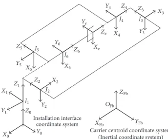
Figure 3: Linkage coordinate frames for a 6-DOF manipulator.
to a proportion of its fitness and individual fitness sum in the whole population. If there are 𝑀𝑐 individuals of the population and the fitness of individual 𝑖 is 𝑓𝑖, then the probability of individual𝑖can be expressed as
𝑃𝑖= 𝑆𝑖
∑𝑀𝑐
𝑘=1𝑆𝑘 (20)
When the selection is given, a random number of 0 to 1 is generated to determine which individuals will cross at next step. The individual which has large selection probability will be selected many times, and its genetic gene will be expanded in the population. On the contrary, it will be eliminated.
Step 4(cross). Select two individuals randomly after selection operation, and a crosspoint of two individuals is generated. By exchanging part of the gene code at the crosspoint, two new individuals are formed.
Step 5 (mutation). According to the probability of gene mutation, the small probability change of binary genetic code of some individuals in the population is realized.
Step 6(new population). The new population is generated by inserting new individuals.
4. Simulation
The simulation object is a typical free-floating 6-DOF space robot, whose reference coordinate system is shown in Fig-ure 3. The linkage parameters𝑎𝑖,𝑏𝑖and the moment of inertia are listed in Table 1. The definition of𝑎𝑖,𝑏𝑖can be referred to in literature [4].
10 15
0 5
Time (s) −0.02
−0.01 0
z
(m/s)
10 15
0 5
0 0.005 0.01
y
(m/s)
10 15
0 5
0 0.005 0.01
x
(m/s)
−0.1 −0.05 0
x
(m/S)
10 15
0 5
−2 −1 0
y
(m/S)
10 15
0 5
−1 −0.5 0
z
(m/S)
10 15
0 5
Time (s)
Figure 4: Desired end-effector velocity of space manipulator end-effector.
Table 1: Linkage parameters of the space robot.
Parameters Carrier Linkage 1 Linkage 2 Linkage 3 Linkage 4 Linkage 5 Linkage 6
Mass (kg) 450.0 1.5 9.6 1.5 9.0 1.5 10.5
𝑎𝑖(mm)
0 0 −492.5 0 292.0 0 −136.0
0 0 54.0 −121.0 −150.0 121.0 0
0 124.0 0 0 0 0 0
𝑏𝑖(mm)
500.0 0 −492.5 124.0 349.0 −124.0 −164.0
0 121.0 −54.0 0 29.0 0 0
751.0 0 0 0 0 0 0
Moment of inertia (kg/m2)
𝐼𝑥𝑥 200.00 3.31×10⁻³ 3.10×10⁻² 3.31×10⁻³ 0.73 3.31×10⁻³ 0.10
𝐼𝑦𝑦 200.00 3.31×10⁻³ 1.50 3.31×10⁻³ 0.60 3.31×10⁻³ 0.10
𝐼𝑧𝑧 200.00 3.31×10⁻³ 1.48 3.31×10⁻³ 0.63 3.31×10⁻³ 0.09
𝐼𝑥𝑦 0 0 0 0 0 0 0
𝐼𝑥𝑧 0 0 0 0 0 0 0
10 15
0 5
Time (s) 0
0.02 0.04 0.06 0.08 0.1 0.12 0.14
De
te
rm
in
an
t o
f G
JM
Figure 5: Determinant of GJM.
10 15
0 5
−5 0 5
−5 0 5
10 15
0 5
−10 0 10
10 15
0 5
time (s)
10 15
0 5
time (s) −200
0 200
10 15
0 5
−200 0 200
10 15
0 5
0 5 10
>6
/>
t(
∘ /M
)
>4
/>
t(
∘ /M
)
>3
/>
t(
∘ /M
)
>2
/>
t(
∘ /M
)
>1
/>
t(
∘ /M
)
>5
/>
t(
∘/M
)
10 20 30 40 50 60 70 80 90 100 0
Generation 0
0.005 0.01 0.015 0.02 0.025 0.03 0.035 0.04
Ob
je
ct
iv
e f
u
nc
tio
n
val
u
e
Minimum value of each generation Average value of each generation
Figure 7: Each generation value of optimization.
0 5 10 15
Time (s)
10 15
0 5
175 180 185
1
(
∘)
−100 −50
3
(
∘)
10 15
0 5
150 200 250
5
(
∘)
10
0 5 15
Time (s) −10
0 10
6
(
∘)
10 15
0 5
−20 0 20
4
(
∘)
10 15
0 5
−100 0 100
2
(
∘)
0 5 10 15
0 5 10 15
10 15
0 5
Time (s)
10 15
0 5
Time (s) −5
0 5
10 15
0 5
−5 0 5
10 15
0 5
0 5 10
0 0.5 1
−5 0 5
−10 −5 0
>6
/>
t(
∘/M
)
>5
/>
t(
∘/M
)
>4
/>
t(
∘/M
)
>3
/>
t(
∘ /M
)
>2
/>
t(
∘/M
)
>1
/>
t(
∘/M
)
Figure 9: The joint velocity path planned by singularity-robust algorithm based on SVD.
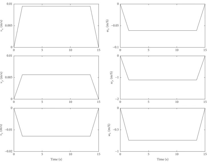
joint angel is 175∘,−60∘,−60∘, 0∘, 210∘, and 5∘. In accordance with the practical sampling period, time step length Δ𝑡 is 250 ms in the simulation. In order to make the motion more smooth, the trapezoidal velocity planning is adopted to the joint motion, as shown in Figure 4.
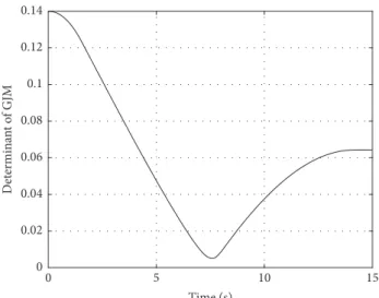
In the calculation of the path planning, the GJM will come across singularity issue. The determinant value of the GJM is close to zero in 7.5 seconds, as shown in Figure 5. If the calculation through the inverse of GJM is still adopted, the joint velocity will become very large (Figure 6), which is unacceptable in practical application, so it is necessary to employ the singular avoidance method.
In the algorithm mentioned in Section 3.2, the parameters of the objective function need to be determined. In (17) and (19), we determine that𝑤1 = 0.5,𝑤2 = 0.5,𝜃+𝑖limit = 6∘/s, and𝜃−𝑖limit=−6∘/s. Through the GA optimization, the value of objective function is improved in each generation, which is shown as in Figure 7. The optimization results are𝜆max= 0.0571𝜀= 0.0677.
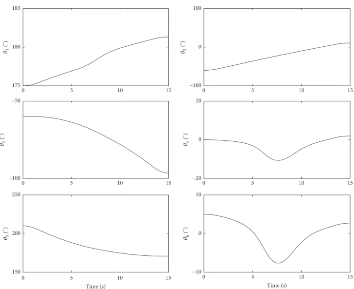
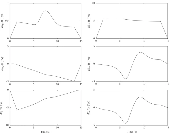
The angle and angular velocity of each joint planned by the adaptive singularity-robust algorithm are shown in Figures 8 and 9, respectively. It can be seen that the joints’
velocity is obviously restricted in the singularity region of GJM when the adaptive and optimized damping is intro-duced in the calculation. The angular velocity of each joint is smooth and the range of each joint velocity is within 6∘/s.
z x
y
Space_Robot Time = 0.0000 Frame = 0001
(a) Time = 0 s
z x
y
Space_Robot Time = 5.0000 Frame = 1001
(b) Time = 5 s
z x
y
Space_Robot Time = 10.0000 Frame = 2001
(c) Time = 10 s
z x
y
Space_Robot Time = 15.0000 Frame = 3001
(d) Time = 15 s
Figure 10: 3D dynamic simulation to the Cartesian path planning for space robot.
have a great influence on the value of optimization objective function, which have a good potential to be optimized. In other directions, the proportion of the errors in the objective function is small, so the effect of optimization is not obvious. If it requires a very strict accuracy in a certain direction, we can achieve the requirements by changing the weight coefficient in the objection function.
5. Conclusions
A space robot can be employed to detect the spacecraft surface through accurate tracking the Cartesian trajectory. It is a typical nonholonomic system, whose Cartesian trajectory planning can only be obtained through the velocity level kine-matics. Therefore, in the path planning based on the inverse GJM, the singularity issue will possibly be encountered. To solve this issue and improve the Cartesian tracking accuracy, the following work is conducted:
(1) The path planning method of Cartesian trajectory planning is given based on the velocity level inverse kinemat-ics model.
(2)Based on the SVD method, the singular avoidance characteristics of GJM are illustrated. The DLS method is improved by introducing an adaptive damping factor which changed with the singularity. For the method introducing a damping, which is adaptively adjusted by𝜆max and𝜀, in the
singular region, the tracking accuracy is not influenced by the singularity-robust algorithm.
(3) In order to improve the tracking accuracy of the singularity-robust algorithm, the objective function includ-ing𝜆maxand𝜀is established, which is optimized by GA.
(4)Through the simulation of a 6-DOF free-floating space robot, the optimized parameters are obtained. Compared with the DLS method, the tracking accuracy of the end-effector is increased by 26.7%.
Data Availability
The modeling data used to support the findings of this study are available from the corresponding author upon request.
Conflicts of Interest
The authors declare that they have no conflicts of interest.
Acknowledgments
×10−3
Adaptive singularity-robust method Damped least square method Adaptive singularity-robust method
Damped least square method
10 15
0 5
Time (s) 0
0.01 0.02
Δp
z
(m)
10 15
0 5
0 2 4
Δp
y
(m)
10 15
0 5
0 0.005 0.01
Δp
x
(m)
0 1 2
Δx
(
∘)
10 15
0 5
0 0.5 1
Δy
(
∘ )
10 15
0 5
0 0.2 0.4
Δ
z
(
∘ )
10 15
0 5
Time (s)
Figure 11: The tracking errors comparisons.
Grant 2014M551231, and Heilongjiang Postdoctoral Fund Grant LBH-Z12131.
References
[1] J. Shi, Y. Cai, and Y. Li, “Research summarizing of on-orbit testing,”Ordnance Industry Automation, vol. 30, no. 6, pp. 59– 62, 2011.
[2] R. Madison, “Micro-satellite based, on-orbit servicing work at the Air Force Research Laboratory,” inProceedings of the 2000 IEEE Aerospace Conference Proceedings, pp. 215–226, Big Sky, MT, USA.
[3] S. E. Fredrickson, S. Duran, and J. D. Mitchell, “Mini AERCam inspection robot for human space missions,” in Proceedings of the A Collection of Technical Papers - AIAA Space 2004 Conference and Exposition, pp. 283–291, San Diego, CA, USA, September 2004.
[4] J. Wu, Y. Zhang, J. Cui, and J. Tan, “Carrier attitude adjustment strategy of a space robot for on-orbit detection,”International Journal of Advanced Robotic Systems, vol. 13, no. 1, Article ID 62246, 2016.
[5] Y. Umetani and K. Yoshida, “Resolved Motion Rate Control of Space Manipulators with Generalized Jacobian Matrix,”IEEE Transactions on Robotics and Automation, vol. 5, no. 3, pp. 303– 314, 1989.
[6] J. Angeles,Fundamentals of Robotic Mechanical Systems: Theory, Methods, and Algorithms, Springer, New York, NY, USA, 2006. [7] Y. Nakamura and H. Hanafusa, “Inverse kinematic solutions with singularity robustness for robot manipulator control,” Journal of Dynamic Systems, Measurement, and Control, vol. 108, no. 3, pp. 163–171, 1986.
[8] C. W. Wampler, “Manipulator inverse kinematic solutions based on vector formulations and damped least-squares methods,” IEEE Transactions on Systems, Man, and Cybernetics, vol. 16, no. 1, pp. 93–101, 1986.
[9] D. Oetomo and M. H. Ang Jr., “Singularity robust algorithm in serial manipulators,”Robotics and Computer-Integrated Manu-facturing, vol. 25, no. 1, pp. 122–134, 2009.
[10] A. S. Deo and I. D. Walker, “Overview of damped least-squares methods for inverse kinematics of robot manipulators,”Journal of Intelligent & Robotic Systems, vol. 14, no. 1, pp. 43–68, 1995. [11] M. G. Carmichael, D. Liu, and K. J. Waldron, “A framework for
singularity-robust manipulator control during physical human-robot interaction,”International Journal of Robotics Research, vol. 36, no. 5-7, pp. 861–876, 2017.
[12] H.-X. Cui, K. Feng, H.-L. Li, and J.-H. Han, “Singularity avoid-ance of 6R decoupled manipulator using improved Gaussian distribution damped reciprocal algorithm,”Industrial Robot: An International Journal, vol. 44, no. 3, pp. 324–332, 2017.
IEEE Transactions on Industrial Electronics, vol. 63, no. 1, pp. 277–290, 2016.
[14] Y.-L. Lai, C.-C. Liao, and Z.-G. Chao, “Inverse kinematics for a novel hybrid parallel–serial five-axis machine tool,”Robotics and Computer-Integrated Manufacturing, vol. 50, pp. 63–79, 2018.
[15] E. Papadopoulos and S. Dubowsky, “Dynamic singularities in the control of free-floating space manipulators,”ASME Journal of Dynamic Systems, Measurement and Control, vol. 115, no. 1, pp. 44–52, 1993.
[16] E. Papadopoulos, “Path Planning For Space Manipulators Exhibiting Nonholonomic Behavior,” in Proceedings of the IEEE/RSJ International Conference on Intelligent Robots and Systems, pp. 669–675, Raleigh, NC, USA, 1992.
[17] R. Lampariello and K. Deutrich, “Simplified path planning for free-floating robots,” DLR Internal Report 515-99-04, 1999. [18] S. Pandey and S. K. Agrawal, “Path Planning of Free-Floating
Prismatic-Jointed Manipulators,”Multibody System Dynamics, vol. 1, no. 1, pp. 127–140, 1997.
Hindawi
www.hindawi.com Volume 2018
Mathematics
Journal ofHindawi
www.hindawi.com Volume 2018
Mathematical Problems in Engineering Applied Mathematics Hindawi
www.hindawi.com Volume 2018
Probability and Statistics Hindawi
www.hindawi.com Volume 2018
Hindawi
www.hindawi.com Volume 2018
Mathematical PhysicsAdvances in
Complex Analysis
Journal ofHindawi
www.hindawi.com Volume 2018
Optimization
Journal ofHindawi
www.hindawi.com Volume 2018
Hindawi
www.hindawi.com Volume 2018
Engineering Mathematics International Journal of
Hindawi
www.hindawi.com Volume 2018
Operations Research
Journal of
Hindawi
www.hindawi.com Volume 2018
Function Spaces
Abstract and Applied Analysis Hindawiwww.hindawi.com Volume 2018
International Journal of Mathematics and Mathematical Sciences
Hindawi
www.hindawi.com Volume 2018
Hindawi Publishing Corporation
http://www.hindawi.com Volume 2013
Hindawi www.hindawi.com
World Journal
Volume 2018
Hindawi
www.hindawi.com Volume 2018Volume 2018
Numerical Analysis
Numerical Analysis
Numerical Analysis
Numerical Analysis
Numerical Analysis
Numerical Analysis
Numerical Analysis
Numerical Analysis
Numerical Analysis
Numerical Analysis
Numerical Analysis
Numerical Analysis
Advances inAdvances in Discrete Dynamics in Nature and Society Hindawiwww.hindawi.com Volume 2018
Hindawi www.hindawi.com
Differential Equations
International Journal of
Volume 2018
Hindawi
www.hindawi.com Volume 2018
Decision Sciences
Hindawi
www.hindawi.com Volume 2018
Analysis
International Journal ofHindawi
www.hindawi.com Volume 2018
![Figure 1 is reproduced from Wu et al. [4]. (2016) (under the Creative Commons Attribution License/public domain)](https://thumb-us.123doks.com/thumbv2/123dok_us/8563741.366439/2.900.467.824.108.397/figure-reproduced-creative-commons-attribution-license-public-domain.webp)