Characterizing representational learning : a combined simulation and tutorial on perturbation theory

Characterizing representational learning: A combined simulation

and tutorial on perturbation theory

Antje Kohnle1,* and Gina Passante2 1

School of Physics and Astronomy, University of St. Andrews, St. Andrews KY16 9SS, United Kingdom 2_{Department of Physics, California State University Fullerton, Fullerton, California 92831, USA}

(Received 24 August 2017; published 28 November 2017)

Analyzing, constructing, and translating between graphical, pictorial, and mathematical representations of physics ideas and reasoning flexibly through them (“representational competence”) is a key character-istic of expertise in physics but is a challenge for learners to develop. Interactive computer simulations and University of Washington style tutorials both have affordances to support representational learning. This article describes work to characterize students’spontaneous use of representations before and after working with a combined simulation and tutorial on first-order energy corrections in the context of quantum-mechanical time-independent perturbation theory. Data were collected from two institutions using pre-, mid-, and post-tests to assess short- and long-term gains. A representational competence level framework was adapted to devise level descriptors for the assessment items. The results indicate an increase in the number of representations used by students and the consistency between them following the combined simulation tutorial. The distributions of representational competence levels suggest a shift from perceptual to semantic use of representations based on their underlying meaning. In terms of activity design, this study illustrates the need to support students in making sense of the representations shown in a simulation and in learning to choose the most appropriate representation for a given task. In terms of characterizing representational abilities, this study illustrates the usefulness of a framework focusing on perceptual, syntactic, and semantic use of representations.

DOI:10.1103/PhysRevPhysEducRes.13.020131

I. INTRODUCTION

Analyzing, constructing, and translating between graphi-cal, pictorial, and mathematical representations of physics ideas, and reasoning flexibly through them is a key character-istic of expertise in physics. Etkinaet al.list“the ability to represent physical processes in multiple ways”as the first of seven key scientific abilities[1]. The ability to work with and translate between representations is a key difference between novice and expert problem solving [2,3]. Different repre-sentations emphasize and deemphasize different aspects of the same concept [4,5], so that fluency in a critical con-stellation of representations may be necessary for deep understanding [6]. The integration of multiple representa-tions can lead to emergent insights into a problem, develop conceptual understanding, and facilitate transfer of knowl-edge across contexts[7]. Understanding multiple represen-tations is necessary for students to make sense of physics textbooks and online materials.

However, abundant research shows that university physics students at all levels have problems employing

representations and using them consistently and reflectively (see, e.g., Refs.[8–10]). Studies have found representation dependent cueing, where features of the representation given in a problem have a significant impact on student success [11–13]. A validated representational fluency survey has shown a distinct gap between low level first year students and more advanced students that use a greater quantity and variety of representations [14–16]. Studies focusing on interactive simulations have found student difficulties with the semantics of the representations shown and the relationships between them[17].

Given the importance of representational abilities and difficulties in attaining them, there is a need to characterize students’ representational abilities and to assess which types of scaffolding support representational learning. A main focus in this paper is to investigate the role of interactive computer simulations in combination with University of Washington style tutorials in developing representational abilities, and to characterize students’ use of representations prior to and after working with these materials using a range of measures.

This article refers to representations as the different external and perceptual forms by which physics concepts can be understood, applied and communicated, such as pictures, diagrams, graphs, tables, text, and mathematics (see, e.g., Ref.[18]for a classification of visual represen-tations). We are interested in students’ use of standard scientific representations rather than their abilities to invent and design new representations (this latter being an aspect *

Corresponding author. [email protected]

of so-called metarepresentational competence[19]). In this article, we define representational competence in terms of the work of Kozma and Russell in chemistry education [20]: this includes (in slightly abbreviated form)

(1) the ability to use representations to describe observ-able phenomena in terms of underlying entities and processes;

(2) the ability to generate or select a representation and explain why it is appropriate for a particular purpose; (3) the ability to identify and analyze features of

representations;

(4) the ability to describe how different representations say the same thing in different ways or something that can not be said with another;

(5) the ability to make connections across different representations and to explain the relationship between them;

(6) to explain how representations correspond to but are distinct from the phenomena they represent; (7) and the ability to use representations and their

features to support claims, draw inferences, and make predictions.

The focus here is primarily on abilities 2, 3, 5, and 7 of this list. Similar to the work by Kohl and Finkelstein[3], the focus is on students’representational abilities in a particular physics context. Thus, the focus is not, for example, on students’abilities with graphs in general, but rather students’ ability to make sense of particular graphs and link them to other representations in a given physics context.

Interactive computer simulations are powerful tools that have been shown to be effective in helping students learn a wide range of physics topics[21]. They often make use of rich static and dynamic visualizations including submicro-scopic domains that can make the invisible visible [22]. Through the design and layout of the simulation features, students can be implicitly guided towards the learning goals[23].

University of Washington style tutorials[24]have been shown to improve students’conceptual understanding[25]. The quantum mechanics tutorial worksheets require stu-dents to engage with some of the most difficult concepts and are scaffolded to guide students through a process that will help them build a more robust, conceptually accurate model for the material [26]. Tutorials are used to supple-ment lectures and take place in small group settings where students work together with a high level of instructor support.

Both simulations and tutorials have particular affordan-ces, and limitations, to support representational learning. Tutorials can elicit prior knowledge of students in a systematic way. They focus on the qualitative interpretation of equations and get students to construct mathematical and graphical representations, analyze their features, and reason through them [27].

Interactive simulations can include multiple representa-tions of the same phenomenon such as text, graphs,

pictures, and mathematics. The interactive elements and dynamical linking of representations can help students make sense of the representations shown and explore the relationships between them. Simulations allow students to quickly explore a large parameter space, reducing the likelihood of students arriving at incorrect conclusions because only a small number of cases have been consid-ered. Simulations can enhance engagement through inter-activity and gamelike features, and can give students direct feedback on their understanding through the displayed quantities and in-built challenges.

In this study we have used a simulation and tutorial in two different ways: as two separate activities, and as a newly developed simulation-tutorial activity designed to employ the affordances of each. The combined simulation-tutorial starts with questions without simulation support focusing on eliciting prior knowledge, interpreting mathematical relations and constructing graphical repre-sentations used in the simulation to support student under-standing of these representations. Students then continue working with the simulation to quickly explore a larger parameter space and get feedback on their understanding, and answer questions with simulation support to extend and generalize their findings.

This study characterizes students’ spontaneous use of representations before and after working with different combinations of a simulation and a tutorial on first-order energy corrections in the context of quantum-mechanical time-independent perturbation theory. This study aims to assess the extent to which students made sense of the representations used in the simulation-tutorial and explic-itly linked representations based on their underlying meaning. Thus, the overall aim was to characterize repre-sentational learning using the materials.

The research questions investigated in the context of quantum-mechanical time-independent perturbation theory include the following:

(1) Can one characterize how students are using repre-sentations via the number and type of representa-tions spontaneously used and the consistency between them?

(2) Can one characterize students’written responses in terms of representational competence levels, and is it possible to measure differences in the distribution of student responses across these levels following targeted instruction?

II. STUDY DESIGN

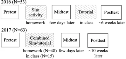
The research study focused on the topic of first-order energy corrections in the context of quantum-mechanical time-independent perturbation theory. The materials devel-oped for the study included an interactive simulation designed to link to the existing University of Washington tutorial on first-order energy corrections; the design of a separate simulation activity and a combined simulation-tutorial; and assessment items for use in the pre-, mid-, and post-tests. The study design and time line of data collection are shown in Fig.1and are discussed in detail below.

Perturbation theory is a powerful technique in quantum mechanics to obtain approximate solutions to potentials that differ only little from ones where the analytical solutions to the Schrödinger equation are known. In first-order time-independent perturbation theory, the correction to the energy eigenvalues is given by Eðn1Þ¼ hnð0ÞjVˆjnð0Þi, where the superscripts 0 and 1 refer to unperturbed and first-order perturbed, respectively, and Vˆ is the perturbation to the potential. For the cases discussed here with a one-dimensional infinite square well of widthLand a perturba-tion that is only a funcperturba-tion of posiperturba-tion, the energy correcperturba-tion is given by an integral that can be reordered to Eðn1Þ¼ R_L

0 VðxÞjψðn0ÞðxÞj2dx. Thus, the first-order energy correction is given by the inner product of the perturbation and the probability density, both of which are functions of position. Note that “energy correction” in this article refers to the first-order energy correction throughout, and that V, ψ, andψ2are used to denoteVðxÞ,ψðxÞ, andψðxÞ2.

The learning goals of the materials used in this study were for students to be able to determine the sign and relative magnitude of the energy correction for a given energy level from the shape of the perturbation and the corresponding probability density, and to use symmetry considerations to explain why some perturbations have zero energy corrections.

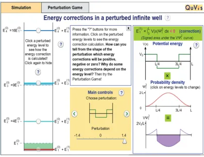
As part of the QuVis Quantum Mechanics Visualization Project[28]we developed an interactive simulation on first-order energy corrections [29] that linked to the existing University of Washington tutorial on this topic [26]. A screenshot of the simulation is shown in Fig. 2. The simulation shows an infinite square well that is perturbed by different potentials, with the energy level diagram on the

left showing the unperturbed and perturbed energy levels as well as the energy correction as the shaded region between them. Students can choose between different perturbations and change their strength via the middle-bottom panel. Students can click on a perturbed energy level to bring up the graphs on the right showing the perturbation V, the probability densityψ2corresponding to the chosen level, and the product graphVψ2, all as a function of position. The top right panel shows the integral expression for the energy correction and the sign of the energy correction. Help buttons (labeled with “?”) bring up short texts explaining the displayed quantities. A second “Perturbation Game” tab asks students to perturb the well so that it absorbs photons of a given energy by choosing both the perturbation shape and strength.

In 2016 we used the University of Washington tutorial on the topic of first-order energy corrections. This tutorial was designed to take an entire 50-min class period after lecture instruction on perturbation theory. The tutorial has students consider several perturbations to the infinite square well. Students are asked to qualitatively reason whether the energy corrections will be positive, negative, or zero.

The simulation activity in both years encouraged explo-ration by asking students to play with the simulation and list three things they had found out about the energy corrections. The activity then aimed to get students to make sense of the representations shown by asking them to make sketches of the energy level diagram and theVψ2product graph and explain these sketches. The activity included questions getting students to reason through the represen-tations, e.g. to explain why a given perturbation has zero energy correction or a positive energy correction for all energy levels. Finally, the activity included questions asking students to make sketches of perturbations different to ones shown in the simulation that fulfilled certain criteria. For example, it asked students to sketch a pertur-bation for which the energy correction of the ground state is greater than that of the first excited state.

For the 2017 combined simulation-tutorial, the activity started with questions without simulation support similar to the start of the original tutorial that asked students to construct representations they would be seeing in the simulation. In this first part, students were asked to interpret the equation for the energy correction, make sketches of the probability densities for the ground state and the first excited state in an infinite square well, to combine the probability density graphs with a simple perturbation that is nonzero only in a small region, and to qualitatively add the perturbed energies to an energy level diagram. The activity then went on to ask students to work with the simulation and answer further questions, similar to the 2016 simu-lation activity. To keep the total 2017 combined simusimu-lation- simulation-tutorial length similar to the 2016 simulation activity, we removed and modified some questions from both the 2016 tutorial and simulation activity.

The combined simulation-tutorial attempts to combine the unique affordances of the simulation and tutorial environments. Having the students engage with the concepts prior to using the simulation elicits their current thinking about the energy correction equation, the graphi-cal interpretation of the wave functions and the perturba-tion potential, as well as the meaning of energy level diagrams. Students are then able to immediately deter-mine if their understanding is correct by interacting with these same representations in the simulation. Including sketching questions builds on the substantial literature of sketching as a successful strategy for learning with text [30,31] and work in chemistry education on sketch-ing to promote representational competence ussketch-ing simu-lations [32].

The simulation and activities were piloted with ten students from the appropriate level (five students in each of 2016 and 2017) in individual volunteer interviews employing a think-aloud protocol. In the 2016 interviews, students were first asked to explore the simulation freely and then work on the associated activity. In the 2017 interviews, students worked on the activity directly, and explored the simulation after working on the initial ques-tions without simulation support. We made revisions to the simulation and activity based on these interviews.

The pre-, mid-, and post-test questions were identical to or similar to those used in a previous study[33]. The pretest questions are shown in Fig.3, and the mid- and post-test questions are shown in Fig. 4. Examples of student responses to the pre- and midtest questions are shown in Fig. 5. The questions provided students with graphical representations of perturbations of a one-dimensional infinite square well and asked qualitative questions about FIG. 2. A screenshot of the“Energy corrections in a perturbed infinite well”simulation.

a V0

Is the first-order correction to the energy for the ground state positive, negative, or zero? Is the first-order correction to the energy for the first-excited state positive, negative, or zero?

For a different perturbation to the square well of width a below:

2.)

3.)

1.) Consider an infinite square well of width a with a delta function pertubation at x = 3a/4. Is the first order correction to the ground state greater than, less than, or equal to the correction to the first excited state?

0

the sign and relative magnitude of the first-order energy correction (Eðn1Þ¼ hnð0ÞjVˆjnð0Þi).

For the questions shown in Figs. 3 and 4, students needed to qualitatively determine the inner product of the given perturbation and the relevant probability density by considering the sign of these functions and their product in terms of the shapes of the relevant graphs. For the first question of the post-test, for example, the ground state probability density ψ2₁ is peaked around the center of the well whereVAis small, but the first excited state probability density ψ2₂ is peaked aroundL=4 and3L=4 where VA is larger. Both energy corrections will be positive, as both the perturbation and the probability density are positive inside the well. However, the product of VA andψ21will have a smaller area under the curve than the product ofVAandψ22. Thus, the energy correction of the ground state will be smaller than that of the first excited state. Answering the pre-, mid-, and post-test questions required students to interpret features of the given perturbation graph, to reason graphically using the formula for the energy correction, and to consider symmetry of the relevant graphs. Thus, the questions probe representational competence related to points 2, 3, 5, and 7 of the representational competence framework in Sec. I.

Figure 1 shows the study design and time line of data collection from a junior-level quantum mechanics course at the University of St. Andrews (United Kingdom) and a senior-level quantum mechanics course at California State Fullerton (CSUF, USA) in 2016 and 2017. The junior- and

senior-level courses are typically taken by students in their third or fourth year. In the junior-level course at St. Andrews, perturbation theory followed discussions of the infinite square well, the harmonic oscillator, and the hydrogen atom in the previous semester. The senior-level course at CSUF used a spins-first approach, and is the second semester of a two-semester quantum mechanics sequence.

In both courses, students completed the pretest after relevant instruction in perturbation theory but prior to working with the materials. In 2016, the pretest questions were given as clicker questions (St. Andrews) and as an online quiz (CSUF). Students then had a few days to complete the simulation activity as a homework assign-ment. In the next lecture, students completed the midtest on paper during 15 min of the lecture period and worked through the tutorial with instructor support. The post-test was part of the midterm assessment for credit. In 2017, the pretest was completed on paper during 15 min of the lecture period. The combined simulation-tutorial was run as a homework assignment (St. Andrews) and as an in-class collaborative activity (CSUF) with students finishing the

V₀

a/2 a

0 0 a/2 a

V₀

a/2 a

0 V₀

a/2 a

0 V0

V_A V_B

Midtest

Posttest

For the potential VA, is the first-order correction to the energy for the ground state greater than, less than, or equal to the first-order correction to the energy for the first-excited state? For the ground state, is the first-order correction to the energy for potential VBgreater than, less than, or equal to the first-order correction to the ground state energy for V_A?

1.)

2.)

FIG. 4. The mid- and post-test questions using two perturbed infinite wells of widtha. Students were given the graphs shown and asked the questions below the graphs, with a prompt to explain their reasoning for each question.

Is the first-order correction to the ground state energy positive, negative, or zero?

Response (a)

Is the first-order correction to the energy for the ground state greater than, less than, or equal to the first-order correction to the energy for the first excited state? Response (b)

Response (c)

a/2 a 0

V₀

a V₀

0

assignment as homework. The midtest was completed in the lecture following the submission of the homework and students were given 15 min to answer. Students were not provided with feedback on pre- and midtest answers.

For the 2017 pretest and the mid- and post-tests across both years, students worked alone and without additional aids. The post-test was part of the final exam. Excepting the post-tests, none of the elements were assessed. However, we have evidence that students took the pre- and midtests seriously, with almost all students taking the entire time allowed and completing all the questions, including pro-viding explanations of their reasoning. There is some evidence that upper-division physics students value these types of formative assessments[34].

Only students completing the activities and the pre-, mid-, and post-tests were included in the study. This led to 53 students (40 St. Andrews and 13 CSUF students) in 2016, and 63 students (48 St. Andrews and 15 CSUF students) in 2017 being included in the study.

Because of the different assessment regimes (unassessed and for credit) and the fact that students may have revised the material for the post-test, it is not possible in this study to compare the efficacy of the different elements. This is, however, not the aim of this paper. Instead, we are interested in devising measures that characterize students’ use of representations, and exploring shifts in these measures following targeted instruction. In Sec. IV, we provide results of statistical tests of difference, as the outcomes provide a baseline for future efficacy studies and demonstrate the usefulness of these measures in ascertaining aspects of representational learning.

III. ANALYSIS METHODS

This study focused on students’ spontaneous use of representations to explain their answer in the pre-, mid-, and post-test questions. For each item, students’responses were coded for correctness of the answer, which repre-sentations were used to justify the answer (text, graphs, mathematics), which graphs were made, and whether or not each representation was used correctly. Representations were only coded for the reasoning to justify an answer, not for the answer itself. The mathematical reasoning code was used for responses including the formula for the energy correction, but not if symbols such asψ,ψ2, orVwere used in text-based reasoning.

Consistency between the representations was coded as consistent, partially consistent (e.g., if three representations were used but only two were consistent) and inconsistent. For example, if a student wrote the correct formula for the energy correction but then incorrectly reasoned using the wave function rather than the probability density, this was coded as inconsistent. Sketches of the wave function were coded as consistent with the energy correction formula and text-based reasoning via the probability density. It is possible for responses to be both consistent and incorrect

(approximately 5% of responses fall into this category). Examples include students that reasoned correctly using the incorrect quantum state (e.g., the first excited state rather than the ground state), and responses without mathematical reasoning that included a sketch of the wave function and text-based reasoning via the inner product ofψandVrather thanψ2andV.

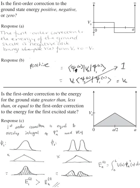
Students’ reasoning was coded as correct if all repre-sentations used were correct and consistent. The examples of student work shown in Fig.5were coded as (a) incorrect text-based reasoning, (b) incorrect mathematical reasoning, and (c) correct and fully consistent text-based, graphical, and mathematical reasoning.

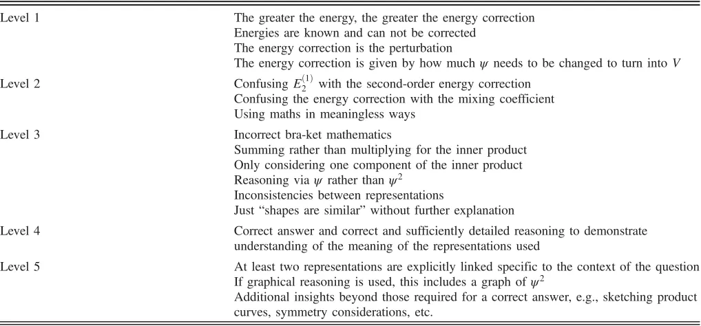
In order to more fully characterize the quality of students’spontaneous use of representations and the links between them, a representational competence level frame-work devised by Kozma and Russell [20] for chemistry education was adapted to devise descriptors for the differ-ent levels for our assessmdiffer-ent items. This framework (see Table 1 in Ref.[20]) consists of five levels, ranging from representation as depiction (level 1), early symbolic skills (level 2), syntactic use of formal representations (level 3), semantic use of formal representations (level 4) and reflective, rhetorical use of formal representations (level 5). Levels 1 and 2 are perceptual in that representations are based only on perceptual features, without regard to syntax or semantics. Level 3 is syntactic, in that formal repre-sentations are used and linked only with a focus on syntactic rules and surface features, not by considering their underlying meaning. Levels 4 and 5 aresemantic, in that formal representations are used and linked by consid-ering their shared underlying meaning. Level 2 includes some symbolic abilities compared with level 1, but still without regard to syntax or semantics. Compared with level 4, level 5 also includes the ability to select and construct the most appropriate representations for a given situation and to explain the relationship between represen-tations. Representations in levels 1, 2, and 3 may not be scientifically accurate.

Figure 5 gives examples of student responses to the assessment items illustrating the different levels. In Fig.5(a), the student states that“The first-order correction to the energy of the ground state is negative as it bringsVðxÞ

from V0 to −V0.” This student seems to see the energy correction as the step in the perturbation in the middle of the well. This answer only focuses on the perceptual features of the graph given in the problem, without regard to the formula for the energy correction or its meaning. Thus, this answer was coded as level 1.

not over the full region. This answer makes use of formal representations, but does not link them to their underlying meaning, e.g., by considering that hereVis a function ofx. Thus, this answer was coded as level 3.

Figure 5(c) shows an answer to one of the midtest questions asking students to compare the energy correc-tions for the ground state and the first excited state for the given perturbation. The student has written the formula for the energy correction, explained the meaning of the formula in words, and made graphs of the probability densitiesψ2, the perturbationV and the productVψ2. The areas below the product curves have been shaded, implying that these areas are used to determine the final result that the ground state energy correction is greater. This answer makes use of correct representations and symbols and explicitly links mathematics, graphs, and text to justify claims. Thus, this answer was coded as level 5.

TableIlists types of responses seen in the assessments and their mapping to representational competence levels. As shown in TableI, a response needed to be fully correct to be coded as level 4 or 5. However, fully correct responses could also be coded as level 3 if the corresponding reasoning was not precise enough. Thus the coding was conservative in that responses were only coded as semantic if they were fully correct with sufficiently detailed explanations that focused on the meaning of the representations used.

A small subset of the data set was coded by both authors to ensure clarity of the code descriptors. The full data set (653 codes per category, 5877 codes in total) was then coded by one of the authors and by an undergraduate student researcher using the given code descriptors. For the repre-sentational competence levels, initial training used the 2017 pre- and midtest and 2016 post-test data, which typically led

to agreement around 68%. Disagreements were discussed prior to a second round of independent coding by the student, which led to the numbers quoted below. For the other codes, no initial training in this form was needed. Comparison of the independent codes for the combined 2016 and 2017 data yielded agreements ranging from 71.1% for the representa-tional competence levels to 96.5% for students’ answers. The use of graphical, text-based, and mathematical reasoning and their consistency yielded agreements of 90.1%, 84.5%, 89.3%, and 80.2%, respectively. For the representational competence levels, only 25 of 653 codes (3.8%) differed by more than one level or were considered to have no reasoning by only one of the coders.

Interrater reliability was also calculated via Cohen’s kappa [35]. For the combined data set, Cohen’s kappa ranged from 0.60 for the representational competence levels to 0.95 for students’answers. The use of graphical, text-based, and mathematical reasoning and their consis-tency yielded kappa values of 0.82, 0.75. 0.76, and 0.72, respectively. In particular, all codes had values of kappa of 0.6 or above, implying satisfactory agreement. To ensure consistency of coding across different types of responses, the percent agreement and Cohen’s kappa were also calculated for the pre-, mid-, and post-tests separately, as well as for the 2016 and 2017 data separately.

In what follows, we present data from both institutions combined. The same trends were seen in the data from the two institutions individually, e.g., an increase in the number of representations used, their consistency, and a shift towards semantic representational competence levels. The mean values for CSUF students were consistently somewhat lower, but in most cases (and in all cases for the midtest results) these differences were not statistically

TABLE I. Descriptors for the different representational competence levels for the pre-, mid-, and post-test responses.

Level 1 The greater the energy, the greater the energy correction

Energies are known and can not be corrected The energy correction is the perturbation

The energy correction is given by how muchψ needs to be changed to turn intoV

Level 2 ConfusingEð₂1Þ with the second-order energy correction

Confusing the energy correction with the mixing coefficient Using maths in meaningless ways

Level 3 Incorrect bra-ket mathematics

Summing rather than multiplying for the inner product Only considering one component of the inner product Reasoning viaψ rather thanψ2

Inconsistencies between representations

Just“shapes are similar”without further explanation

Level 4 Correct answer and correct and sufficiently detailed reasoning to demonstrate

understanding of the meaning of the representations used

Level 5 At least two representations are explicitly linked specific to the context of the question

If graphical reasoning is used, this includes a graph ofψ2

significant. For example, the percentage of correct answer and reasoning in the 2017 pre-, mid-, and post-tests were 4.4%, 56.7%, and 50% for CSUF students, and 22.9%, 60.4%, and 58.3% for St. Andrews students. As another example, the mean number of representations used in the 2017 pre-, mid-, and post-tests were 0.87, 1.37, and 1.87 for CSUF students, and 1.35, 1.56, and 2.32 for St. Andrews students. Given the similar trends seen in the data from both institutions, the focus of this article on shifts between the assessments rather than differences between the two groups of students, and the relatively small student numbers involved (40 St. Andrews and 13 CSUF students in 2016, and 48 St. Andrews, and 15 CSUF students in 2017), the data presented here is from both institutions combined. In Sec. IV, all results of statistical significance tests are reported for two-tailed tests.

IV. RESULTS

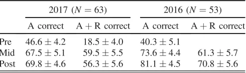
The main focus of this article is on students’ use of representations. For completeness, the average percent of students with correct answers and both correct answer and reasoning are given in TableII. Reasoning was considered correct if the mathematical, graphical, and/or text-based reasoning used in a given response were all correct. Note that no reasoning data for the 2016 pretest was available.

A. Number and types of representations

This section discusses research question 1: “Can one characterize how students are using representations via the number and type of representations spontaneously used and the consistency between them?”The mean number of representations used per assessment item is shown in TableIII. The increase in the mean number of representa-tions between the 2017 pre- and midtest is significant (t¼3.079, df¼62, p¼0.003, d¼0.49), with a medium effect sized. The mean number of representations used in the 2016 midtest was similar to the 2017 midtest. Across both years, the mean number of representations in the post-tests were significantly higher than in the midtests (for 2017,t¼7.744,df¼62,p <0.0005,d¼1.28; for 2016, t¼5.523, df¼52, p <0.0005, d¼0.91). The greater number of representations in the post-tests may possibly be due to the framing of the post-tests as part an

assessment for credit compared with no credit being given for the pre- and midtests.

There is substantial variation in student success depend-ing on whether or not graphs were made and the types of graphs made. Thus, this section looks in more detail at the graphical representations used in students’ reasoning. TableIV shows the types of graphs made by students for the 2016 and 2017 assessment items. The Table is divided into no graph, graphs of the wave functionψ (that some-times also included a graph of the perturbation V), and graphs of the probability densityψ2 (that sometimes also included graphs of ψ and V). A very small number of students (5 in total) just sketched the perturbation that is given in the problem and were grouped into“no graph”in the table. Comparing the 2017 pre- and midtests in the table (the first two data columns), the fraction of responses with a graph increased from the pre- to the midtest (t¼2.469,

df¼62, p¼0.016, d¼0.39). The mid- and post-test results in Table IV are similar across both years. The fraction of students making graphs was greater in the post-tests than in the midpost-tests (for 2017, t¼2.942, df¼62,

p¼0.005, d¼0.50; for 2016, t¼2.748, df¼52,

p¼0.008,d¼0.43), possibly due to the assessed nature of the post-test compared with the unassessed pre- and midtests. TableIValso shows a shift in the types of graphs made by students from mostly wave function graphs in the pretest to mostly probability density graphs in the midtest. In the post-tests, more students in total made a sketch compared with the midtest, but the fraction of students making sketches of the probability densityψ2was similar to the midtests.

TABLE II. The mean percentage of correct responses for the pre-, mid-, and post-tests, considering only students’answers (A) and considering both answer and reasoning (AþR). Errors are the standard errors on the mean.

2017 (N¼63) 2016 (N¼53)

A correct AþR correct A correct AþR correct

Pre 46.64.2 18.54.0 40.35.1

Mid 67.55.1 59.55.5 73.64.4 61.35.7 Post 69.84.6 56.35.6 81.14.5 70.85.6

TABLE III. The mean number of representations (graphs, mathematics, text) used per assessment item in the pre-, mid-, and post-test responses. Errors are the standard errors on the mean.

2017 (N¼63) 2016 (N¼53)

Pre Mid Post Mid Post

Mean number of representations

1.24 1.52 2.21 1.65 2.10

0.07 0.07 0.06 0.07 0.07

TABLE IV. The percentage of responses in the pre-, mid-, and post-test responses with no graph (“None”), graphs of the wave function ψ (that sometimes also included a graph of the perturbationV), and graphs of the probability densityψ2 (that sometimes also included graphs of ψ and V). Errors are the standard errors on the mean.

2017 (N¼63) 2016 (N¼53)

Pre Mid Post Mid Post

None 75.23.9 57.15.4 37.34.7 50.05.7 34.04.6

ψ 20.63.6 7.22.7 25.44.5 8.53.2 22.64.8

In the situations discussed in the materials, the first-order energy correction is given by the inner product of the perturbation and the probability density. Thus, a sketch of the probability density is generally more productive than a sketch of the wave function, which requires a mental construction of the probability density to reason correctly about the first-order energy correction using shapes or symmetry. Table V considers the correctness of students’ responses in relation to the graphical representations used. The top row of TableVshows that responses that included a sketch of ψ2 were far more likely to have the correct answer and reasoning than responses that had no sketch or only included a sketch ofψ. The top row of TableValso indicates that responses that included a sketch of ψ were less likely to be correct compared with responses that included no sketch or a sketch of ψ2. It is possible that sketchingψ leads students astray in their answers or that an incorrect interpretation of the formula leads students to sketchψ and reason incorrectly.

A common type of error seen in∼8%of responses to the assessment items was reasoning viaψ rather thanψ2. For example, for the perturbation with odd symmetry shown at the top of Fig.5, students would incorrectly state that the energy correction for the first excited state is positive, as the product ofVandψwill be positive for allxand thus the signed area under the product curve is positive. The middle row of TableVsuggests a correlation between sketchingψ and this type of incorrect reasoning, as a higher fraction of responses that sketchedψ showed this error compared with responses with no sketch or with a sketch of ψ2.

B. Consistency between representations

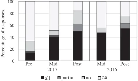
Inconsistent use of representations in a given response may indicate that students are not able to correctly interpret the representations or not translate between them based on their underlying meanings. Figure6shows the percentage of responses with fully consistent, partially consistent (i.e., two of three representations are consistent) and inconsistent use of representations across the pre-, mid-, and post-test items. Each question on the assessments was counted individually in these distributions. Code “na” was used for students’ responses with only a single representation or with no reasoning.

Comparing the 2017 pre- and midtests in Fig.6(the two left-most columns), one can see an increase in the con-sistency between representations and an increase in the fraction of responses using multiple representations. Comparing the 2017 mid- and post-tests in Fig. 6 (the second and third left-most columns), one can see an increase in the fraction of responses using multiple repre-sentations, but little change in the fraction of fully con-sistent responses, with more inconcon-sistent or partially consistent responses. A similar trend is seen comparing the 2016 mid- and post-tests.

In order to assess the statistical significance of the results, zero points were mapped to a single representation or inconsistent representations (na and“no”in Fig.6), one point to partially consistent representations (“partial” in Fig.6) and two points to fully consistent representations (“all”in Fig.6). A Wilcoxon matched-pairs signed-ranks test was carried out on the mean consistency values for each student for pairs of assessment items. The difference between the 2017 pre- and midtests was significant (z¼3.774,

N-ties¼18,p <0.0005), whereas the difference between the mid- and post-tests were marginally not significant across both years (for 2017z¼1.825,N-ties¼18,p¼0.07; for 2016z¼1.902,N-ties¼20,p¼0.06).

TABLE V. The percentage of responses with both correct answer and reasoning (top row) and the percentage of incorrect responses usingψrather thanψ2in the inner product to calculate the energy correction (middle row), separated into students that made no graph, a graph ofψ, and a graphψ2as for TableIV. The bottom row shows the number of responses used to determine each of the percentages. The mid- and post-test results were combined over both years.

Midtest (2016/17) Post-test (2016/17)

No graph ψ graph ψ2 graph No graph ψ graph ψ2 graph

Percentage answer and reasoning correct 47.2 38.9 83.1 60.2 39.3 79.6

Percentage with incorrectψ reasoning 4.8 33.3 1.1 8.4 30.3 0.0

Number of responses 125 18 89 83 56 93

0 20 40 60 80 100

all partial no na

2017 2016

Pre Mid Post Mid Post

Percentage of responses

C. Characterizing representational competence

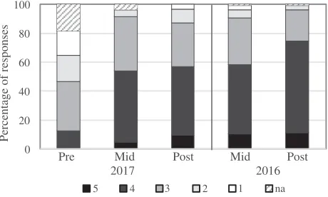
This section focuses on research question 2: “Can one characterize students’ written responses in terms of repre-sentational competence levels, and is it possible to measure differences in the distribution of student responses across these levels following targeted instruction?” Section III describes the coding scheme for representational competence levels for the assessment items. Figure7shows the distri-butions across the representational competence levels for the pre-, mid-, and posttest questions. The 2016 pretest did not include reasoning, so that only the 2017 pretest is shown in the figure. Each question on the assessments was counted individually in these distributions. Code na was used if there was no reasoning for a given assessment item.

In 2017, students completed the combined simulation-tutorial between the pre- and the midtest. Figure7 shows that the 2017 pretest distribution has a greater fraction of perceptual responses (codes 1 and 2) and lower fraction of semantic responses (codes 4 and 5) than the 2017 midtest distribution. A Wilcoxon matched-pairs signed-ranks test was carried out on the mean representational competence levels for each student for the pre- and midtest. Responses with no reasoning were not included in the mean. The increase between the 2017 pre- and midtest levels was significant (z¼5.795, N-ties¼11, p <0.0005). The 2017 mid- and post-test level distributions are very similar. In 2016, students worked on the University of Washington tutorial between the mid- and the post-test. Figure 7 shows that the 2016 post-test distribution has a greater fraction of semantic responses (codes 4 and 5) than the 2016 midtest distribution. A Wilcoxon test similar to the one above showed a significant increase between the mid-and post-test levels (z¼2.642, N-ties¼18, p¼0.008). The 2016 post-test results have a greater fraction of semantic reasoning compared with 2017 (U¼1305.0,

N1¼53, N2¼63, p¼0.033), but students in 2016 had more instruction (the stand-alone simulation assignment

and the tutorial) compared with 2017 (only the combined simulation-tutorial).

V. DISCUSSION

The focus of this study was whether students are able to make sense of the representations developed in the simu-lation-tutorial and successfully make links between them. Students used a greater number of representations in the assessment items in the 2017 midtest compared with the pretest. However, the number of representations alone does not fully characterize students’representational abilities, as it does not include how these representations are used. Kohl and Finkelstein[3]found that novices and experts differed little in the quantity of representation used (albeit the students studied came from representation-rich PER-informed courses), but rather in how these representations were used. Experts used representations to make sense of the physics, whereas unsuccessful novices made representations out of a sense of requirement and not toward any particular purpose. Hill and Sharma[15] found differences between students with low and high representational fluency in the number and variety of representations used, their coherence, and the quantity of visual and symbolic representations. Our study used the consistency between representations in students’reasoning and representational competence levels adapted from the framework of Kozma and Russell [20] to characterize how students were using representations. Inconsistent use of representations was assumed to indicate that students were not making sense of representations or not connecting them based on their underlying meaning.

This study found an increase in the consistency between representations from the 2017 pre- to midtest, and a shift from perceptual to semantic reasoning as measured by the representational competence levels. Thus, both the consis-tency between representations and the representational competence levels point to a shift towards greater semantic use of representations after the simulation-tutorial. For the 2017 post-test compared with the midtest, there was a significant increase in the number of representations used, but little difference in the fraction of responses with fully consistent use of representations and little difference in the distribution over representational competence levels. The fraction of fully correct answers also did not increase. The framing of the post-test as an assessment for credit may have led to greater representation use, but it did not lead to a greater semantic use of representations. Thus, this study shows the need to consider how representations are used and not just their number to characterize representation abilities. The ability to choose the most appropriate representation for a given task is one aspect of representational compe-tence (see point 2 in Sec.I). In this study, student responses showed a correlation between correctness and the use of particular representations. There were large differences in correctness for responses that included probability density graphs compared with those that did not. Responses with a

0 20 40 60 80 100

1 2 3 4

5 na

2017 2016

Pre Mid Post Mid Post

Percentage of responses

wave function graph were less likely to have correct reasoning compared with responses with no graph or a probability density graph. Some of the responses with a wave function graph incorrectly reasoned via the wave function rather than the probability density to determine the energy correction. One interpretation of these results is that probability density graphs are particularly productive in qualitative reasoning about energy corrections, as they reduce cognitive load in reasoning about the inner product of V and ψ2 that yields the energy correction. Having graphs of both components of the inner product visible (the graph ofVwas given in the problem text) reduces cognitive load compared with having only the graph of one compo-nent visible or needing to mentally square a sketched wave function graph. There is also some indication that the wave function graph leads students astray to argue via the symmetry of V and ψ, as a number of responses that incorrectly reason via the inner product ofVandψdirectly make reference to the symmetry of ψ as shown in their sketch. The materials developed for this study focus on representations that are productive in qualitative reasoning about energy corrections. This study shows the need to support students in learning to choose the most appropriate representation for a given task.

Students’ responses were characterized in terms of perceptual, syntactic and semantic representational com-petence levels. The distribution of students’responses over these levels characterized changes in students’ use of representations between the pre-, mid-, and post-test. This study demonstrates the implementation of a frame-work focusing on perceptual, syntactic and semantic use of representations for characterizing representational learning and changes in representational competence throughout instruction. This framework may be useful for many other contexts as a way to characterize representations and representational competence.

There are a number of limitations of this work. This study only considered students’spontaneous use of repre-sentations in qualitative reasoning, and did not include assessment items testing specific representational abilities such as sketching the product function for two given curves. Only 47 of 464 responses (10%) in the mid- and post-tests included sketches of the product of the pertur-bation and the probability density, and only 32 of these 47 responses (68%) were correct. For the St. Andrews students completing the 2017 simulation-tutorial as homework, 67% were successful at creating the product graph in the initial problems without simulation support. For CSUF students completing the 2017 simulation-tutorial in class with instructor support, this fraction was 100%. This indicates that scaffolding is needed to support students’ representa-tional abilities to sketch a product function, and that assessment items testing for this ability could be useful. It may also be useful to ask students to reflect on and improve the graphs they constructed prior to simulation use

when the combined simulation-tutorial is implemented as homework and not in class with instructor support.

As the 2016 pretest did not include students’reasoning, it is not possible to directly compare the efficacy of the 2016 simulation activity with the 2017 combined simulation-tutorial.

This study shows the need to support students in learning to choose the most appropriate representation for a given task. While the simulation-tutorial focuses solely on prob-ability density and not on the wave function, a small number of students still sketched the wave function in the midtests and reasoned incorrectly, and a substantial number of students made no sketch. Future work aims to include reflective questions in the combined simulation-tutorial getting students to reflect on which representations are most useful for qualitative reasoning about the energy corrections. The representational competence level descriptors adapted to the assessment items were found to be suffi-ciently reliable. However, the definitions of the levels and their use with written responses have limitations. Our coding was conservative in that responses needed to be fully correct to be characterized as semantic (levels 4 and 5). This, however, led to some responses that were quite detailed and almost correct still being categorized as syntactic (level 3). Such answers may be more appropri-ately described as a mixture of semantic and syntactic reasoning, whereas the level descriptors are exclusive. Also, while semantic use of representations characterizes expert practice, syntactic use of representations when fully correct may not distinguish between experts and novices, as experts may also use syntactic reasoning for routine tasks. Thus, interviews that provide more details on students’ thought processes and allow a fuller characterization of perceptual, syntactic or semantic reasoning would be useful to complement this study.

VI. CONCLUSION

In conclusion, this study has characterized students’ responses in terms of the number and types of representations used, and perceptual, syntactic, and semantic representa-tional competence levels to assess changes in students’use of representations. Following the simulation-tutorial, stu-dents’responses showed a shift from perceptual to semantic reasoning, and an increase in the number of representations used and the consistency between them.

This study has implications for the design of activities to support representational learning with interactive simula-tions. Students need to be supported in making sense of and constructing the representations used in the simulation, and reflect on which representations are most useful for a given task.

this study may be useful for a wide range of contexts to characterize and assess changes in representational abilities and for comparative studies of the effectiveness of resources in enhancing representational competence.

ACKNOWLEDGMENTS

The authors would like to thank Nicola Pinzani and Sam Lloyd for the coding of the simulation, and all students that

participated in the evaluation studies and provided feedback on the materials. We would like to acknowledge the work of Alexander Jackson on initial analysis of the 2016 data. We thank Chao Dun Tan for coding the full data set to test for reliability. We thank the University of St. Andrews for funding the development of simulations. The authors would like to thank Shaaron Ainsworth for useful discussions and helpful feedback on a draft of this manuscript.

[1] E. Etkina, A. Van Heuvelen, S. White-Brahmia, D. T. Brookes, M. Gentile, S. Murthy, D. Rosengrant, and A. Warren, Scientific abilities and their assessment,Phys. Rev. ST Phys. Educ. Res.2, 020103 (2006).

[2] R. J. Dufresne, W. J. Gerace, and W. J. Leonard, Solving physics problems with multiple representations, Phys. Teach.35, 270 (1997).

[3] P. B. Kohl and N. D. Finkelstein, Patterns of multiple representation use by experts and novices during physics problem solving, Phys. Rev. ST Phys. Educ. Res. 4, 010111 (2008).

[4] J. Zhang and D. A. Norman, Representations in distributed cognitive tasks,Cogn. Sci. 18, 87 (1994).

[5] O. Parnafes and A. Disessa, Relations between types of reasoning and computational representations, Int. J. Comput.9, 251 (2004).

[6] J. Airey and C. Linder, A disciplinary discourse perspec-tive on university science learning: Achieving fluency in a critical constellation of modes,J. Res. Sci. Teach. 46, 27 (2009).

[7] S. Ainsworth, DeFT: A conceptual framework for consid-ering learning with multiple representations,Learn. Instr.

16, 183 (2006).

[8] L. C. McDermott, M. L. Rosenquist, and E. H. Van Zee, Student difficulties in connecting graphs and physics: Examples from kinematics, Am. J. Phys. 55, 503 (1987).

[9] E. Gire and E. Price, Structural features of algebraic quantum notations,Phys. Rev. ST Phys. Educ. Res. 11, 020109 (2015).

[10] A. Maries, S. Y. Lin, and C. Singh, Challenges in designing appropriate scaffolding to improve students’ representa-tional consistency: The case of a Gauss’s law problem,

Phys. Rev. Phys. Educ. Res.13, 020103 (2017). [11] P. B. Kohl and N. D. Finkelstein, Student representational

competence and self-assessment when solving physics problems, Phys. Rev. ST Phys. Educ. Res. 1, 010104 (2005).

[12] D. E. Meltzer, Relation between students’problem-solving performance and representational format,Am. J. Phys.73, 463 (2005).

[13] M. De Cock, Representation use and strategy choice in physics problem solving,Phys. Rev. ST Phys. Educ. Res.

8, 020117 (2012).

[14] M. Hill, M. Sharma, J. O’Byrne, and J. Airey, Developing and evaluating a survey for representational fluency in science, Int. J. Innov. Sci. Math. Educ.22, 22 (2014). [15] M. Hill and M. D. Sharma, Students’ representational

fluency at university: a cross-sectional measure of how multiple representations are used by physics students using the Representational Fluency Survey, Eurasia J. Math. Sci. Technol. Educ.11, 1633 (2015).

[16] M. Hill, M. D. Sharma, and H. Johnston, How online learning modules can improve the representational fluency and conceptual understanding of university physics stu-dents,Eur. J. Phys. 36, 045019 (2015).

[17] V. Lòpez and R. Pintó, Identifying secondary-school students’difficulties when reading visual representations displayed in physics simulations,Int. J. Sci. Educ.39, 1353 (2017).

[18] G. L. Lohse, K. Biolsi, N. Walker, and H. H. Rueter, A classification of visual representations,Commun. ACM37, 36 (1994).

[19] A. A. diSessa, Metarepresentation: Native competence and targets for instruction, Cognit. Instr.22, 293 (2004). [20] R. Kozma and J. Russell, Students becoming chemists:

Developing representational competence, inVisualization in science education, edited by J. K. Gilbert (Springer, Dordrecht, 2005), p. 121.

[21] N. Rutten, W. R. Van Joolingen, and J. T. Van der Veen, The learning effects of computer simulations in science education,Comput. Educ.58, 136 (2012).

[22] A. Kohnle, C. Baily, A. Campbell, N. Korolkova, and M. Paetkau, Enhancing student learning of two-level quantum systems with interactive simulations,Am. J. Phys.83, 560 (2015).

[23] N. S. Podolefsky, K. K. Perkins, and W. K. Adams, Factors promoting engaged exploration with computer simulations,

Phys. Rev. ST Phys. Educ. Res.6, 020117 (2010). [24] L. C. McDermott, P. S. Shaffer, and the U. W. Physics

Education Group,Tutorials in Introductory Physics, 1st ed. (Prentice Hall, Upper Saddle River, 2002).

[25] N. D. Finkelstein and S. J. Pollock, Replicating and under-standing successful innovations: Implementing tutorials in introductory physics, Phys. Rev. ST Phys. Educ. Res.1, 010101 (2005).

[27] L. C. McDermott, Millikan Award Lecture: What we teach and what is learned—Closing the gap,Am. J. Phys.59, 301 (1991).

[28] The Quantum Mechanics Visualization Project (Online);

https://www.st-andrews.ac.uk/physics/quvis/ [5 July 2017].

[29] Energy Corrections in a Perturbed Infinite Well (Online);

https://www.st-andrews.ac.uk/physics/quvis/simulations_ html5/sims/perturbationGame/perturbationGame.html [5 July 2017].

[30] S. Ainsworth, V. Prain, and R. Tytler, Drawing to learn in science,Science333, 1096 (2011).

[31] P. Van Meter and J. Garner, The promise and practice of learner-generated drawing: Literature review and synthesis,

Educ. Psychol. Rev.17, 285 (2005).

[32] M. Stieff, Improving representational competence using molecular simulations embedded in inquiry activities,

J. Res. Sci. Teach.48, 1137 (2011).

[33] G. Passante, P. J. Emigh, T. Wang, and P. S. Shaffer, Investigating student understanding of perturbation theory and inner products of functions, in Proceedings of the Physics Education Conference Proceedings 2015, College Park, MD, edited by A. D. Churukian, D. L. Jones, and L. Ding (AIP, New York, 2015), p. 247.

[34] M. E. Loverude, Assessment to complement research-based instruction in upper-level physics courses,AIP Conf. Proc.1413, 51 (2012).