Flux and Speed Estimation of Induction Motors using Extended Kalman Filter

Flux and Speed Estimation of Induction Motors using

Extended Kalman Filter

Osamah Basheer Noori

MSc student at Department of Electrical

Engineering,

Colloage of Engineering,University of

Mosul

Mohammed Obaid Mustafa,

PhD

Lecturer at Department of Electrical Engineering,

Colloage of Engineering, University of Mosul

ABSTRACT

The application of the field-oriented control strategy to induction motors needs the knowledge of the rotor flux components. On the other hand, in order to enhance the performance of sensorless control of induction motor, the rotor flux and speed of the induction motor should be known. Therefore

In this article and based on the fifth order nonlinear model of the induction motor, the rotor flux and speed of induction motor are being estimated simultaneously using the Extended Kalman Filter (EKF) algorithm. Multiple simulation results are being presented that prove the efficacy of the proposed scheme towards flux and speed estimation of induction motor.

General Terms

Adaptive Control and Decision Supporting Systems.

Keywords

Extended Kalman filter, Estimation of speed and rotor flux, Induction motor,Model of induction motor.

1.

INTRODUCTION

Induction motors are essential components in the vast majority of industrial processes, while due to the fact that these motors are operating in difficult working environments, there are numerous degrading factors such as: dust, temperature variations, humidity, continuous operation, and heavy loads. In the last decade the problem of achieving high performance from induction motor - with sensorless control - is a very interesting topic [1].

On the other hand, Field-Oriented Control (FOC) allows high performance speed and torque response to be achieved from an induction motor. The instantaneous magnitude and position of the rotor flux space vector must continuously be known with precision in order to achieve and maintain perfect field orientation. This can be achieved by using a nonlinear state observer [2].

FOC can have a good performance and low maintenance with high torque obtained as compared to traditional methods such as V/F and E/f. FOC needs a rotor flux of induction motor, in this paper, the Extended Kalman filter has been proposed for obtaining the rotor flux through estimation[2].

It is well-known that most control systems for the Induction Motor (IM) require the knowledge of the rotor fluxes as well as that of the angular speed [3]. Since these measurements, in particular those of the fluxes, are not easily accessible, many research efforts have been focused on their estimation in the past few years.

Indeed, many alternatives have been studied in order to design observers for IM using Luenberger-like observer [4], [5], nonlinear observers [6], sliding mode-based observer [7]. However, in most of these works, the speed measurement has

been supposed to be available and the objective of these works was to provide on-line estimates of the rotor fluxes only.

In this paper, the estimation of rotor flux and speed for the IM is carried out. The considered model accounts for five state variables, namely the two stator currents, the two rotor fluxes, and the motor speed. The objective of the estimation scheme is to estimate from the current calculations. Then, an appropriate state observer that provides.

The rest of the article is being structured as it follows: In Section 2 the model derivation and simplification, for the induction motor is being derived. In Section 3, discrete model of induction motor is being stated, followed by the proposed Kalman filtering in Section 4. Section 5 contains simulation results, while the conclusions are drawn in the last ,Section 6.

2.

MODEL OF INDUCTION MOTOR

Because it is highly nonlinear, thus requiring much more complex control algorithms, induction machine was traditionally, and for a long time, used in fixed speed applications for reasons of cost, reliability and efficiency. With this machine, the torque and flux are controlled independently, thus allowing fast torque response and high precision of regulation to be achieved[8].

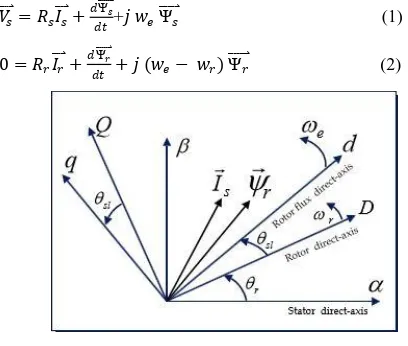
Figure 1, shows the 𝑑 − 𝑞 coordinate system rotating at speed (𝜔𝑒). The mathematical model of induction motor, in space vector notation, is given by the following equations[9]:

𝑉𝑠

= 𝑅_𝑠𝐼 +𝑠 𝑑Ψ 𝑠

𝑑𝑡+𝑗 𝑤𝑒Ψ 𝑠 (1)

0 = 𝑅𝑟𝐼 +𝑟 𝑑Ψ 𝑟

𝑑𝑡 + 𝑗 (𝑤𝑒− 𝑤𝑟) Ψ 𝑟 (2)

Fig 1: Reference frames and space vectors

The stator flux space vector Ψ 𝑠 , the rotor flux space vector Ψ_𝑟

and the electromagnetic torque are given by equations (3), (4) and (5) below, where 𝐼 𝑠, 𝐼 𝑟 are the stator and the rotor current respectively:

Ψ_𝑠

28 Ψ𝑟

= 𝐿𝑚𝐼 + 𝐿𝑠 𝑟𝐼 𝑟 (4)

𝑇𝑒= 3𝑝𝐿_2𝐿𝑚

𝑟 (Ψ ∗ 𝐼𝑟 )𝑠 (5)

Using the 𝛼 − 𝛽 coordinate system (stationary reference frame) and separating the machine variables into their real and imaginary parts, the well-known induction motor model expressed in term's of the state variables is obtained from (1) to (5) and is given by the equation (6) below [8,9,10]:

𝑑 𝑑𝑡 𝐼𝑠𝛼 𝐼𝑠𝛽 Ψ𝑟𝛼 Ψ_𝑟𝛽 𝜔𝑟 =

− 𝜎𝐿𝑅𝑠𝑠+

1−𝜎 𝜎 𝜏𝑟 𝐼𝑠𝛼+

𝐿𝑚

𝜎 𝐿𝑠𝐿𝑟𝜏𝑟Ψ𝑟𝛼+

𝐿𝑚𝜔𝑟

𝜎 𝐿𝑠𝐿𝑟Ψ𝑟𝛽 +

1 𝜎 𝐿𝑠𝑉𝑠𝛼

− 𝑅𝑠

𝜎 𝐿𝑠+

1−𝜎 𝜎 𝜏𝑟 𝐼𝑠𝛽−

𝐿𝑚𝜔𝑟

𝜎 𝐿𝑠𝐿𝑟Ψ𝑟𝛼+

𝐿𝑚

𝜎 𝐿𝑠𝐿𝑟𝜏𝑟Ψ𝑟𝛽 +

1 𝜎 𝐿𝑠𝑉𝑠𝛽

𝐿𝑚

𝜏𝑟𝐼𝑠𝛼−

1

𝜏𝑟Ψ𝑟𝛼− 𝜔𝑟Ψ𝑟𝛽

𝐿𝑚

𝜏𝑟𝐼𝑠𝛽−

1

𝜏𝑟Ψ𝑟𝛽 + 𝜔𝑟Ψ𝑟𝛼

3𝑝2_𝐿 𝑚

2𝐽𝐿𝑟 𝐼𝑠𝛽Ψ𝑟𝛼 − 𝐼𝑠𝛼Ψ𝑟𝛽 −

𝐹 𝐽𝜔𝑟−

𝑝 𝐽𝑇𝑙

(6)

In equation (6), 𝜎 is the coefficient of dispersion and is given by equation (7) below:

𝜎 = 1 −

(𝐿𝑠𝐿𝑟)

(7)

3.

DISCRETE MODEL OF INDUCTION

MOTOR

In order to obtain the discrete model of induction motor , we have to transform the continuous model of IM to discrete one by using discretization methods ,one of them is the Euler transformation. The discrete model of IM can be written as follows [8,9]:

𝐼𝑠𝛼(𝑘 + 1)

𝐼𝑠𝛽(𝑘 + 1

𝜑𝑟𝛼(𝑘 + 1)

𝜑𝑟𝛽(𝑘 + 1)

𝜔𝑟(𝑘 + 1)

=

(𝑎1− 𝑎2

1 𝑡𝑟 𝑘

𝐼𝑠𝛼 𝑘 + 𝑎3

1 𝑡𝑟 𝑘

𝜑𝑟𝛼 𝑘 + 𝑎3𝜑𝑟𝛽 𝑘 𝜔𝑟 𝑘 + 𝑎𝑠𝑉𝑠𝛼(𝑘)

(𝑎1− 𝑎2

1 𝑡𝑟 𝑘

𝐼𝑠𝛽 𝑘 + 𝑎3

1 𝑡𝑟 𝑘

𝜑𝑟𝛽 𝑘 − 𝑎3𝜑𝑟𝛼(𝑘)𝜔𝑟 𝑘 + 𝑎𝑠𝑉𝑠𝛽(𝑘)

𝑎3

1 𝑡𝑟 𝑘

𝐼𝑠𝛼 𝑘 + 1 −

Δ𝑡 𝑡𝑟 𝑘

𝜑𝑟𝛼 𝑘 −Δ𝑡𝜔𝑟(𝑘)𝜑𝑟𝛽(𝑘)

𝑎3

1 𝑡𝑟 𝑘

𝐼𝑠𝛽 𝑘 + 1 −

Δ𝑡 𝑡𝑟 𝑘

𝜑𝑟𝛽 𝑘 +Δ𝑡𝜔𝑟(𝑘)𝜑𝑟𝛼(𝑘)

𝑎6 𝐼𝑠𝛽 𝑘 𝜑𝑟𝛼 𝑘 − 𝐼𝑠𝛼 𝑘 𝜑𝑟𝛽 𝑘 + 𝑎6𝜔𝑟(𝑘)

(8)

Where:

𝑎1= 1 − 𝑎0𝑅𝑠𝐿𝑟Δ𝑡

𝑎2= 𝑎0 𝐿𝑚2Δ𝑡

𝑎3= 𝑎0 𝐿𝑚Δ𝑡

𝑎4= 𝑎0 𝐿𝑚

𝑎5= 𝑎0 𝐿𝑟Δ𝑡

𝑎6=

3𝑝2_𝐿 𝑚Δ𝑡

2𝐽𝐿𝑟

𝑎7= {1 −

𝐹Δ𝑡 𝐽 −

𝑝Δ𝑡𝑇𝑚𝑎𝑥

𝐽𝑤𝑟.𝑚𝑎𝑥

}

𝑎0=

1 ( 𝐿𝑠 𝐿𝑟− 𝐿𝑚2)

In above equations, 𝛥𝑡 represents the length of the sampling interval. Obviously, the smaller 𝛥𝑡 is better the Euler approximation is; otherwise this requires a fast microprocessor system for the on-line implementation of the filter. The employment of a stochastic approach overcomes in part these difficulties, because it intrinsically takes into account the model mismatching and therefore a not very small length 𝛥𝑡 can be chosen.

4.

KALMAN FILTERING

The Kalman filter is an estimation tool used in many branches of engineering and science. The Kalman filter is recursive mean algorithm which is capable of estimating the unknown states depending on information of measured ones [11]. The filter estimation is obtained from the predicted values of the states and this is corrected recursively by using a correction term, which is the product of the Kalman gain and the deviation of the estimated measurement output vector and the actual output vector. The Kalman gain is chosen to result in the best possible estimated states.

4.1

Linear Kalman Filter (KF)

The KF can be introduced by considering the linear discrete time system described by the state space equations [12]:

𝑥 𝑘 + 1 = 𝐹 𝑘 𝑥 𝑘 + 𝐺 𝑘 𝑢 𝑘 + 𝑤 𝑘 (9)

𝑦 𝑘 = 𝐻 𝑘 𝑥(𝑘) + 𝑣(𝑘) (10) where 𝑥 (𝑘)is the state vector, 𝑦 (𝑘) is the output or measurement vector and 𝑢 𝑘 is the known input. Also 𝐹 𝑘 ,

𝐺 𝑘 and 𝐻 𝑘 are the system, input and output or measurement matrices respectively , Furthermore, 𝑤 𝑘 and

𝑣(𝑘)represent the system and measurement noises characterized by:

𝐸 𝑤 𝑘 = 𝑂. 𝐸 𝑣 𝑘 = 𝑂. ∀ 𝑘 𝐸 𝑤 𝑘 𝑤𝑇 _{𝑗 = 𝑄 𝑘 𝛿}

𝑘𝑗 𝑄 ≥ 0 (11)

𝐸[𝑣 𝑘 𝑣𝑇 _{𝑗 ] = 𝑅 𝑘 𝛿}

𝑘𝑗 𝑅 > 0

𝐸 𝑤 𝑘 𝑣𝑇 _{𝑗 = 𝑂. ∀ 𝑘j}

where 𝛿𝑘𝑗is the Kronecker delta. The initial state 𝑥(0)is an independent random vector with known statistics.

𝐸 𝑥 0 = 𝑥0 . 𝐸[(𝑥(0) − 𝑥0 )(𝑥(0) − 𝑥0 )𝑇] = 𝑃0 (12) The problem is to find an estimate 𝑥(𝑘/𝑘) of the state 𝑥(𝑘)at time 𝑘 with its error covariance 𝑃(𝑘/𝑘) = 𝐸[(𝑥(𝑘) − 𝑥 𝑘/𝑘 (𝑥(𝑘) − 𝑥(𝑘/𝑘))𝑇_{] . The notation 𝑥(𝑘/𝑘)implies the} estimate, is to be based on all the measurements obtained up to and including 𝑦(𝑘)obtained at time 𝑘. The equations for the Kalman filter are:

𝑥 𝑘 + 1/𝑘 = 𝐹 𝑘 𝑥 𝑘/𝑘 + 𝐺 𝑘 𝑢 𝑘 (13)

𝑃 𝑘 + 1/𝑘 = 𝐹 𝑘 𝑃 𝑘/𝑘 𝐹𝑇_{(𝑘) + 𝑄(𝑘) (14)}

𝑥 (𝑘 + 1/𝑘 + 1) = 𝑥(𝑘 + 1/𝑘) + 𝐾(𝑘 + 1)[𝑦(𝑕1) − 𝐻 𝑘 + 1 𝑥(𝑘 + 1/𝑘)] (15)

𝐾 𝑘 + 1 = 𝑃 𝑘 + 1/𝑘 𝐻𝑇 _{𝑘 + 1 [𝐻 𝑘 + 1 𝑃 𝑘 +}

1/𝑘 𝐻𝑇 _{𝑘 + 1 + 𝑅 𝑘 + 1 ]}−1 ₍₁₆₎

𝑥 (0/0) = 𝑋𝑜; 𝑃(0/0) = 𝑃𝑜 (18)

4.2

Extended Kalman Filter (EKF)

To use KF with non linear system models it is necessary to first linearize the model about a nominal or auxiliary state trajectory to produce a linear perturbation model. The basic KF is used to estimate the perturbation states and then these are combined with the auxiliary states to produce the state estimates of the non linear model. When the auxiliary state is made equal to the most recent KF estimate the procedure is known as the Extended Kalman Filter (EKF). The EKF can be applied as a state estimator for non linear systems. It can carry out combined state and parameter estimation treating selected parameters as extra states and forming an augmented state vector. The result is that whether the original state space model was linear or not the augmented model will be non linear because of multiplication of states.

Let the non linear model of the system be described by the following equations [13]:

𝑥(𝑘 + 1) = 𝑓(𝑥 𝑘 , 𝑢 𝑘 ) + 𝑤(𝑘) (19)

𝑌 𝑘 = 𝐻 𝑘 𝑥(𝑘) + 𝑣(𝑘) (20) where 𝑥 𝑘 , 𝑌 𝑘 and 𝑢 𝑘 are respectively the state, the measurement and the input vectors; 𝑓(𝑥 𝑘 , 𝑢 𝑘 ) is a vector state function of state vector and 𝐻 𝑘 is the measurement matrix. Furthermore, 𝑤(𝑘) and 𝑣(𝑘) represent the system and measurement noises with statistic described by Eqs. (11).The equations of EKF are :

𝑥(𝑘 + 1/𝑘) = 𝑓(𝑥 𝑘 , 𝑢 𝑘 ) (21) Φ(𝑘) = 𝜕

𝜕𝑋𝑓(𝑥 𝑘/𝑘 . 𝑢 𝑘 ) 𝑥(𝑘)−𝑥(𝑘/𝑘) (22)

𝑃 𝑘 + 1/𝑘 =Φ 𝑘 𝑃 𝑘/𝑘 Φ𝑇_{(𝑘) + 𝑄(𝑘) (23)}

𝑥(𝑘 + 1/𝑘 + 1) = 𝑥(𝑘 + 1/𝑘) + 𝐾 (𝑘 + 1) [𝑦 𝑘 + 1 − 𝐻 𝑘 + 1 𝑥 𝑘 + 1/𝑘 ] (24)

𝐾(𝑘 + 1) = 𝑃 𝑘 + 1/𝑘 𝐻𝑇 𝑘 + 1 [𝑅(𝑘) + 𝐻(𝑘 +

1)𝑃(𝑘 + 1/𝑘) 𝐻𝑇 _{(𝑘 + 1)]} −1 ₍₂₅₎

𝑃(𝑘 + 1/𝑘 + 1) = [𝐼 − 𝐾 𝑘 + 1 𝐻 𝑘 + 1 ]𝑃(𝑘 + 1/𝑘) (26)

𝑥(0/0) = 𝑥0; 𝑃(0/0) = 𝑃0 (27) In general the EKF is not optimal and, due to the linear approximation, it is possible for the estimates to diverge so that care must be taken in its application. In some case, it is convenient to use the following rather than Eq. (26) :

𝑃 (𝑘 + 1/𝑘 + 1) = [𝐼 − 𝐾(𝑘 + 1) 𝐻 (𝑘 + 1)) 𝑃 (𝑘 + 1/𝑘) 𝐼 − 𝐾 𝑘 + 1 𝐻 𝑘 + 1 −1_{+ 𝐾(𝑘 + 1)𝑅(𝑘 +}

1)𝐾𝑇_{(𝑘 + 1) (28)} In order to apply extended Kalman filter on induction motor ,we have to define the state transition equations of the induction motor as follows[1]:

𝑋(𝑘 + 1) = 𝑓(𝑋 𝑘 , 𝑈 𝑘 , 𝑘) + 𝑊 𝑘 (29)

𝑌(𝑘) = 𝑕(𝑋 𝑘 , 𝑘) + 𝑉(𝑘) (30) Where 𝑋 𝑘 , 𝑈 𝑘 , 𝑌(𝑘) , are respectively at time 𝑘 ,the state vector, the input vector (𝛼 − 𝛽 components of the stator voltage space vector), the output vector (𝛼 − 𝛽 components of the stator voltage space vector)

𝑋 𝑘 = [𝐼𝑠𝛼(𝑘) 𝐼𝑠𝛽(𝑘) 𝜑𝑟𝛼(𝑘) 𝜑𝑟𝛽(𝑘) 𝜔𝑟(𝑘)]𝑇 (31)

𝑈 𝑘 = [𝑉𝑠𝛼(𝑘) 𝑉𝑠𝛽(𝑘)]𝑇 (32)

𝑌 𝑘 = [𝐼𝑠𝛼(𝑘) 𝐼𝑠𝛽(𝑘)]𝑇 (33)

𝑊 𝑘 and 𝑉(𝑘) are random vectors, and are respectively the process and the measurement noise vectors.

where 𝐹 is the jacobian matrix of the plant due to states and

𝐺 is the jacobian matrix of plant due to inputs.

𝐹 = 𝜕

𝜕𝑋𝑓(𝑋 𝑘 , 𝑈 𝑘 ) 𝑋(𝑘) (34)

𝐺 = _𝜕𝑈𝜕 𝑓(𝑋 𝑘 , 𝑈 𝑘 )

𝑋 𝑘 ,𝑈(𝑘) (35)

5.

SIMULATION RESULTS

The suggested scheme of EKF for flux and speed estimation of induction motor is being evaluated on a model of three phase induction motor having the parameters depicted in Table 1.

𝑅 = 𝑑𝑖𝑎𝑔([0.1, 0.1])

𝑄 = 𝑑𝑖𝑎𝑔( 2𝑥10−2_{, 2𝑥10}−2_{, 2𝑥10}−3_{, 2𝑥10}−3_{, 1 )}

𝑃 = 𝑑𝑖𝑎𝑔( 1𝑥10−2_{, 1𝑥10}−2_{, 1𝑥10}−1_{, 1𝑥10}−1_{, 10 )} Table 1. Parameters of induction motor

Parameters Value

𝑃𝑟𝑎𝑡𝑒𝑑 1.1 kw

𝑉𝑁 380 V

𝐼𝑁 2.7 A

𝐹𝑁 50 Hz

𝑇𝑙 7.5 N.m

𝐽 0.02 kg.𝑚2

𝑛𝑁 1410 r/min

𝑅𝑠 5.27 Ω

𝑅𝑟 5.07 Ω

𝐿𝑚 0.421 H

𝐿𝑠 0.423 H

𝐿𝑟 0.479 H

𝜎𝐿𝑠 0.053 H

𝑃 (pole pair) 2

𝛥𝑡 (sec) 50∗ 10−6

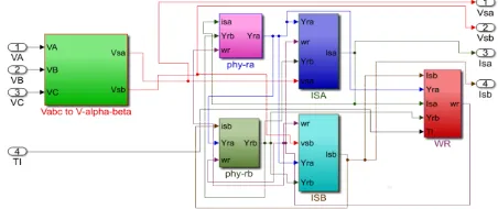
Figure 2 is presented the model of induction motor while figure 3 is being presented EKF estimator. Figure 4 shows the simulation set up for estimation of rotor speed and flux of induction motor along with stator currents and voltages.

30 Fig 3: Model of Extended Kalman Filter estimator

Fig 4: Matlab simulation set up for estimation of rotor flux and speed

By using MATLAB/Simulink, the model of induction motor has been constructed and then the EKF estimator applied on it. The first simulation results present the actual and estimated speed of induction motor as it is being presented in figure (5). As it can be observed from figure 3, the results shown that the EKF has good tracking performances for motor speed.

Fig 5: Estimated and actual rotor speed Nr (rpm)

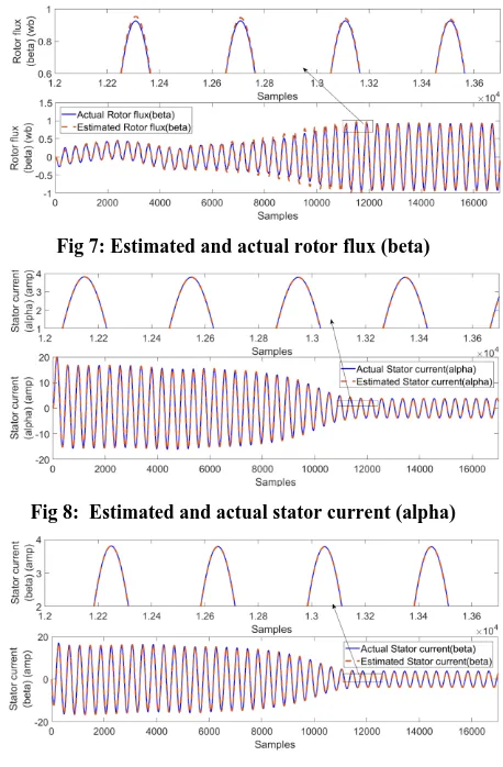
The figure 6 and figure 7 form simulation results, will focus in presenting the difference between the motor’s estimated flux and actual flux (flux (alpha) and flux (beta) ) respectively. it is clear that the estimated value follows the actual value. Thus using EKF we are getting an optimal estimator of motor flux.

Fig 6: Estimated and actual rotor flux (alpha)

In the sequence the simulation results on the figures (8-9) shows that a good tracking performance is achieved and the above results demonstrate that the proposed method has strong efficacy for estimating the stator current Isa and Isb components.

Fig 7: Estimated and actual rotor flux (beta)

Fig 8: Estimated and actual stator current (alpha)

Fig 9: Estimated and actual stator current (beta)

6.

CONCLUSIONS

In this article and based on the fifth order nonlinear model of the induction motor, the rotor flux and speed of induction motor are being estimated simultaneously using the Extended Kalman Filter (EKF) algorithm.

The suggested scheme has the capability for estimating the speed (𝜔𝑟) and the rotor flux of induction motor by combining information from the induction motor model along with output to produce an optimal state of the motor. Multiple simulation results have been presented that proved the efficiency of the proposed scheme for state estimation of three phase induction motor

.

7.

REFERENCES

[1] G. G. Acosta, C. J. Verucchi, and E. R. Gelso, , “ current monitoring system for diagnosing electrical failures in induction motors ,” Mechanical Systems and Signal Processing, vol. 20, no. 4, pp. 953-965, Oct 2004. [2] F. Blaschke, , “The Principle of Field Orientation as

Applied to the New Transvektor Closed-Loop Control System for Rotating-Field Machines,” Siemens Review (5), 1972, 217-219.

[3] W. Leonard, Control of electrical drives. 3rd edition. , Springer- Verlag, 2001.

[5] Ph. Martin and P. Rouchon , “Two simple flux observers for induction motors,” International Journal of adaptive control and signal processing, 14 (2/3):171–176, 2000. [6] K. Busawon, H. Yahoui, H. Hammouri, and G. Grellet , “

A nonlinear observer for induction motors,” The European Physical Journal Applied Physics, 15:181–188, 2001.

[7] A. Benchaib, A. Rachid, E. Audrezet, and M. Tadjine , “Real-time sliding-mode observer and control of an induction motor,” IEEE Trans. Ind. Electron., 46(1):128– 138, 1999.

[8] Mohand A., Ouhrouche, “ Estimation Of Speed, Rotor Flux And Rotor Resistance In Cage Induction Motor Using The Ekf Algorithm,” International Journal of Power and Energy Systems 2002.

[9] P. Vas, Electrical Machines and Drives: A Space Vector Theory Approach, New York, Oxford University Press, 1992.

[10]P. Vas, Vector Control of AC Machines, New York, Oxford University Press, 1990.

[11]A. Bennassar, a. Abbou, m. Akherraz, “ speed sensorless indirect field oriented control of induction motor using an extended kalman filter ,” Journal of Electrical Engineering.

[12]Pietro Muraca, Ciro Picardi , “a reduced order extended kalman filter algorithm for parameter and state estimation of an induction motor ,” IFAC Proceeding, Volume 25,Issue 20,September 1992, Pages 255-230. [13]L. Rossignol, M. Farza, and M. M’Saad, “ Nonlinear