Strong sesquiterpene emissions from Amazonian soils

Strong sesquiterpene emissions from Amazonian

soils

E. Bourtsoukidis

1

, T. Behrendt

2

, A.M. Yañez-Serrano

1,3,8

, H. Hellén

4

, E. Diamantopoulos

5

, E. Catão

2

,

K. Ashworth

6

, A. Pozzer

1

, C.A. Quesada

3

, D.L. Martins

3,9

, M. Sá

3

, A. Araujo

3

, J. Brito

7,10

, P. Artaxo

7

,

J. Kesselmeier

1

, J. Lelieveld

1

& J. Williams

1

The Amazon rainforest is the world’s largest source of reactive volatile isoprenoids to the

atmosphere. It is generally assumed that these emissions are products of photosynthetically

driven secondary metabolism and released from the rainforest canopy from where they

in

fl

uence the oxidative capacity of the atmosphere. However, recent measurements indicate

that further sources of volatiles are present. Here we show that soil microorganisms are a

strong, unaccounted source of highly reactive and previously unreported sesquiterpenes

(C

15

H

24

; SQT). The emission rate and chemical speciation of soil SQTs were determined as a

function of soil moisture, oxygen, and rRNA transcript abundance in the laboratory. Based on

these results, a model was developed to predict soil

–

atmosphere SQT

fl

uxes. It was found

SQT emissions from a Terra Firme soil in the dry season were in comparable magnitude to

current global model canopy emissions, establishing an important ecological connection

between soil microbes and atmospherically relevant SQTs.

DOI: 10.1038/s41467-018-04658-y

OPEN

1_{Atmospheric Chemistry and Biogeochemistry Departments, Max Planck Institute for Chemistry, Hahn-Meitner-Weg 1, 55128 Mainz, Germany.}2_Max Planck Institute for Biogeochemistry, Hans-Knöll-Straße 10, 07745 Jena, Germany.3National Institute of Amazonian Research, Av. André Araújo, 2936 -Petrópolis, Manaus, AM 69067-375, Brazil.4Finnish Meteorological Institute, Erik Palménin aukio 1, FI-00560 Helsinki, Finland.5Department of Plant and Environmental Science, University of Copenhagen, Thorvaldsensvej 40, 1871 Frederiksberg C, DK-1871 Copenhagen, Denmark.6Lancaster Environment Centre, Lancaster University, Lancaster LA1 4YQ, UK.7_{University of Sao Paulo, Rua do Matão, Travessa R, 187, São Paulo, SP CEP 05508-900, Brazil.} 8_{Present address: University of Freiburg, Georges-Köhler-Allee 53, 79110 Freiburg, Germany.}9_{Present address: Imperial College London, London SW7 2AZ,} UK.10_{Present address: Laboratory of Atmospheric Physics (LaMP), University Blaise Pascal, 63000 Clermont-Ferrand, France. Correspondence and requests} for materials should be addressed to E.B. (email:e.bourtsoukidis@mpic.de)

123456789

S

esquiterpenes are a chemically diverse class of volatile

iso-prenoids relevant to biology, ecology, and due to their high

reactivity to ozone and prodigious particle production

ef

fi

ciency to atmospheric composition

1–5

. They are known to be

emitted to the air from plants as a function of oxidative and

thermal stress

6–9

. By generating strong spatial gradients, due to

their rapid reaction with ozone, they may affect olfactory

navi-gation in pollinating insects

10

.

The substantial diversity of species within this compound class,

the rapid reaction with ozone, the low ambient mixing ratios, and

the low volatility make it dif

fi

cult to quantify them accurately and to

elucidate impacts within the ecosystem

8,11,12

. Current

fl

ux

para-meterizations are formulated based on scarce measurements from

plant systems only, uni

fi

ed with an empirical temperature response

for all the species in the family

13,14

. Although some sesquiterpenes

have been detected previously in soil

15–18

, the relevance of this

source to the atmosphere is unclear. In particular, carbon-rich

tropical soils, which have not been examined previously

19

, could be

potent but overlooked sources.

In this study, we use a laboratory-derived emission algorithm to

evaluate the impact of Amazonian soils on the net ecosystem SQT

fl

ux and hence atmospheric chemistry. We combine proton

transfer

–

mass

spectrometry

(PTR-MS)

and

gas

chromatography

–

mass spectrometry (GC-MS) methods to evaluate

the soil SQT emission strength in the laboratory and in the

fi

eld.

The laboratory incubations reveal strong emissions of SQTs from

soils as a function of water-

fi

lled pore space (WFPS), allowing the

development of an emission algorithm that was validated with

fi

eld

samples. Simulated results compared closely with SQT

fl

ux

mea-surements in the

fi

eld, so a two-year period (2014

–

2015), was

modeled based on in situ rainfall and soil moisture measurements.

The simulations indicate that SQT emissions from soils are in

comparable magnitude with canopy emissions while they dominate

O

3

reactivity in the forest

fl

oor.

Results

Laboratory observations

. To quantify and chemically speciate

SQT emission

fl

uxes, 42 soil samples were collected at three

depths from eight Amazonian sites (Supplementary Table

1

). The

samples included Ferralsols, Alisols, and Podzols, originating

from three major ecosystems: dense Terra Firme forest (TF),

fl

oodplain terrace (FLT), and white sand (WS). While most of TF

soils investigated are in the pristine Amazonian forest in the

vicinity of the Amazonian tall tower observatory (ATTO), TF4

and TF5 are located at the ecotone of rainforest to cerrado

(tropical savanna ecoregion) and were part of the large-scale,

long-term

fi

re experiment

20

. The soils were selected on the basis

of type to represent the majority of soils in the Amazon basin

21

.

In all laboratory-based experiments, the soil atmosphere was

simulated by mixing environmentally relevant VOC ratios and

CO

2

either into zero air or pressurized N

2

to simulate aerobic and

anaerobic conditions, respectively. At the beginning of each

experiment, the soils were wetted to 100% water-

fi

lled pore space

(WFPS) and allowed to desiccate in a controlled and continuously

monitored environment

22

.

Upon the initial wetting, a strong burst release of SQTs was

observed for the majority (>80 %) of the incubated soils from TF

and FLT but not from WS. Following the initial burst directly

after wetting, soil VOC emissions in the laboratory stabilized and

2

–

3 days later SQTs (C

15

H

24

) and acetone (C

3

H

6

O) displayed

clear and reproducible optima as a function of soil moisture

(Fig.

1

). Such emission optima have been previously linked to

microbial activity for NO and HONO

23,24

over similar moisture

ranges

(WFPS

SQT,opt.

=

31.3 ± 6.3%,

WFPS

acetone,opt.

=

10.2 ±

2.7%). Acetone emissions were the strongest, with release rates

up to 1.5 mg m

2

h

−1

; an order of magnitude higher than acetone

net

fl

uxes measured above an Amazonian forest

25

. However, the

WFPS over which the acetone emissions occur is signi

fi

cantly

lower than conditions normally experienced in the Amazonian

rainforest. Contrasting behavior was reproducibly exhibited by

methanol, which was weakly up-taken under wet conditions and

released during drying, while monoterpenes were (in contrast

Nor

maliz

ed flux

Atmosphere

Organic (0) hor

iz on T o psoil (A) Subsoil (B) 100

100 67 35 13 4

0.6

0.3

0

0–5 cm : aerobic

0–5 cm : anaerobic

100 200

0

0 24 48 72 96

1.8 1.2 0.6 600 400 200 0 –100 100 20 10 0 –5 20 0 –20 –40

100 71 44 16

66 34 10 3

0 Time (h)

0 24 48 72 96

0.4

0.2

0

–0.2 Time (h)

0 24 48 72 96

Time (h)

0 24 48 72 96

Time (h) –50

80 60 40 20 0

WFPS (%)

WFPS (%)

100 67 41 23

WFPS (%)

WFPS (%)

WFPS (%)

F (

μ g m –2 h –1 )

F (

μ g m –2 h –1 )

F (

μ g m –2 h –1 )

F (

μ g m –2 h –1 ) F acet

. (mg m

–2 h –1 ) F acet

. (mg m

–2 h –1 ) F acet.,MT ,meth.,aa (mg m –2 h –1 )

10–15 cm : anaerobic

45–50 cm : anaerobic*

Total SQT Acetone Total MT Methanol (m205) (m59) (m137) (m33) α -gurjunene α -himachalene α -bergamontene α -f ar nesene γ

-gurjunene _β-hum

with the canopy

fl

uxes

25

) weakly emitted under wet conditions

and moderately consumed in the low-moisture range.

Besides soil moisture, which consistently produced an emission

optimum, the most important environmental factors driving SQT

production and release were found to be the soil type, depth, and

oxygen availability. Temperature only weakly increased SQT

emission, as has been noted previously for Mediterranean soils

26

,

while varying CO

2

abundance (400

–

5000 ppm

v

) had no effect on

the emission pattern or strength. Substantial differences in SQT

release were observed from the different sub-ecosystems and soil

horizons (Figs.

2

and

3

). An order of magnitude stronger

emission rate was measured for the TF1 ecosystem. Terra Firme

soils (TF1, TF2, and TF3) have very similar physiochemical

properties (pH, bulk density, total reserve bases (

Σ

RB

), clay

content) and similar morphological properties

27

. Such a

sub-stantial difference in the SQT emission rates between TF1 and the

other two Terra Firme sites may be attributable to a higher

microbial activity.

To investigate a link between microbial activity and SQT

emissions, subsamples of soil were collected during soil

desicca-tion experiments from TF4 to TF5 and 16S- to 18S rRNA

transcript abundances (indicator for bacterial and fungal activity,

respectively) were quanti

fi

ed at three points: (1) upon wetting, (2)

during the optimum, and (3) under dry conditions. TF4 and TF5

belong to the southern part of the Amazonian rainforest and have

been shown to be the least fertile but are widespread across

eastern Amazonia

28

and were subject to a long-term

fi

re

experiment

20

. TF4 is located in the natural forest (control area)

and TF5 in the area that was burned every 3 years (B3Yr) during

the experiment (2004

–

2010). As shown in Fig.

4

, SQT emissions

were reproducibly high for TF4 and 16S rRNA transcript

abundance displayed an optimum at similar soil moisture as

the maximum of SQT emissions. In contrast, TF5 (burned site)

showed negligible emissions of SQTs and the respective 16S

rRNA transcript abundance was up to three orders of magnitude

less and invariant over all samples. The 18S rRNA transcript

abundance was equally high during the optimum for both soils,

indicating that the role of fungal emissions is insigni

fi

cant relative

to bacterial SQT emissions for these soils. Despite the limitations

that may arise from the use of rRNA as an indicator of microbial

activity

29

, both the ecological history and rRNA dynamics

observed indicate that the microbial activity drive the SQT

production and release for these soils. TF4 and TF5 are typical for

a drier region of the Amazonian basin and in addition, SQT

emissions from fungi are strongly dependent on fungal-age,

rather than biomass

30

. Therefore, the bacterial/fungal

contribu-tion to the net SQT produccontribu-tion in the Amazon basin requires

further investigation, particularly as a function of season and

fungal development stage.

In the absence of oxygen, stronger VOC emissions are

expected

31

. This is indeed the case for SQT emissions from the

organic (O) horizon (Fig.

3

). Along with the production strength,

the chemical diversity of SQT emissions increased (see Fig.

1

c and

Supplementary Fig.

1

). While only four SQT species were

measured from TF1 under aerobic conditions (

α

- and

β

-gurjunene,

α

-himachalene, and

α

/

β

-cubebene), in the absence of

oxygen, a total of ten different SQTs were released and the

emission ratios have changed markedly. A correspondingly broad

spectrum of SQT was identi

fi

ed from the topsoil (A) horizon

(10

–

15 cm). Field samples at TF1 contained the species that were

seen only under anaerobic conditions in the laboratory (see

Fig.

1

a and Table

1

). This is a clear indication that the uppermost

aerobic organic (O) horizon is not the only source for the SQTs

entering the atmosphere, and that the subsurface layer

con-tributes to the emission

fl

ux since SQTs can rapidly travel up

through soil with very small losses

32

.

Emission algorithm

. The emissions observed in the laboratory

are the result of conditions commonly occurring in nature. A

natural rain event initiates a cascade of physiochemical and

microbial processes as the water percolates through the soil layers.

After the rain, the SQT emission burst declines exponentially and

then stabilizes as the optimum-shaped microbial emissions start

to increase. Therefore, the emission dynamics could be divided

into two distinct ranges of soil moisture: a high moisture regime

(HM; see cyan area in Fig.

5

a, b) up to

≈

80% WFPS and a

moderate moisture regime (MM; beige area) from

≈

80% WFPS to

complete desiccation. We combined these two processes into a

single equation that can be used for the quanti

fi

cation of SQT

soil-to-atmosphere

fl

uxes in all environments and under both

aerobic and anaerobic conditions (Fig.

5

a, b). The emission model

algorithm was applied in all laboratory experiments, where an

emission optimum was observed for a particular WFPS. Close

agreement between the emission algorithm and measured

emis-sions (0.89 <

R

2

< 0.97) indicates that the algorithm can reliably

simulate the observed SQT emissions (see example in Fig.

5

a, b).

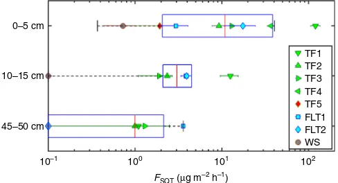
Fig. 1Vertical profile of VOCfluxes from a Terra Firme soil (TF1).a

Normalized soil_fluxes of sesquiterpenes (SQTs) (red) and acetone (purple) as a function of water-filled pore space (WFPS). The normalized (to the optimum emission observed at moderate moisture) algorithm-derived emission curve is the result of integrating laboratory observations fromb

organic horizon under aerobic andcanaerobic conditions,dtopsoil (10–15 cm) andesubsoil (45–50 cm). SQTs, monoterpenes (MTs), acetone, and methanol are illustrated with the colored lines. Acetone, methanol, and_α -pinene were included in the fumigation standard (see Methods). The shaded areas indicate the standard deviation of the measured emission rates at each chamber cycle. The pie charts illustrate the chemical speciation of SQT at the point in time (and WFPS), indicated by the white circle over the SQT measurements (red line). For the color scale, see lower right panel. The pie chart ataillustrates the chemical composition under

field conditions. The asterisk inedenotes that the experiments were performed under aerobic conditions despite the predominant anaerobic conditions in the deep soil layers

0–5 cm

10–15 cm

45–50 cm

10–1 ₁₀0 ₁₀1 ₁₀2

TF1 TF2 TF3 TF4 TF5 FLT1 FLT2 WS

FSQT (μg m–2 h–1)

[image:3.595.306.550.483.615.2]

Field measurements

. To evaluate the algorithm,

fl

ux

measure-ments were made in the

fi

eld using Te

fl

on chambers placed

directly on the surface soil at TF1 and TF3 (ATTO site).

Volu-metric soil water content is continuously monitored at the ATTO

site with six sensors, arranged vertically from 10 to 100 cm depth.

Hydrological modeling and in situ volumetric moisture

mea-surements were combined to derive the WFPS in the

fi

eld. In our

model for SQT emissions from Amazonian soils, we use the

−

3

and

−

10 cm WFPS to predict

fi

eld emissions by integrating the

emission burst from anaerobic (O) horizon and the microbial

emissions from both aerobic (O) and anaerobic (A) horizons

(Fig.

5

c). Our model considers anaerobic conditions for the

fi

rst

few hours after a strong rainfall event under the HM regime. It

has been shown that it is dif

fi

cult to predict the O

2

availability

after rainfall since soil O

2

is not a direct function of rain water

33

.

Our

fi

eld measurements quanti

fi

ed exceptionally strong emissions

of SQT, 6 h after strong rainfall (25.1 mm in 2 h). These emissions

were stronger than our model prediction, indicating that either

the emission burst could be stronger compared with the

labora-tory observations or that the topsoil (A) signi

fi

cantly contributes

to anaerobic emission burst. We note that according to our

hydrological model, topsoil (A) is very rarely under anaerobic

conditions and hence such conditions were not included in the

emission model. The chemical speciation of the

fi

rst sample was

very different from the following samples along the natural

desiccation process with bergamontene and isocaryophyllene

comprising more than 90% of the total SQT detected up to 6 h

after the rainfall. The rest of the samples contained a mixture of

103

102

101

100

1 2 3 4 5 6 7 8 9 10 11 12 13

Sample number

14 15 16 17 18 19 20 21 22 23 24 25 TF1

Anaer.

Anaer. Anaer.

F

Anaer. Anaer.

TF2 TF3 TF4 TF5 FLT1 FLT2 WS

FSQT

(

μ

g m

–2 h

–1

)

Fig. 3Organic (O) horizon (0–5cm) SQT emissions during a complete dry out. All experiments started from saturated moisture conditions. The data represent the emission rates measured with WFPS >10% apart from the samples S5, S8, S11, and S12 that dried up to WFPS≈45%. On each box, the center line (red) indicates the median, and the bottom and top borders of the box (blue) indicate the 25th and 75th percentiles, respectively. The whiskers extend to the most extreme data points not considered outliers, and the outliers are plotted individually using the“+”symbol (red). The boxplot draws points as outliers if they are greater than q3_+w× (q3_–q1) or less than q1_–w× (q3_–q1). q1 and q3 are the 25th and 75th percentiles of the sample data, respectively. The“Whisker”(w) corresponds to ±2.7σand 99.3% coverage if the data are normally distributed. The green markers indicate the optimum SQTflux (inμg m−2h−1). The large boxes around S5, S8, S11, S19, and S22 indicate that these experiments were conducted under anaerobic conditions. The symbol F indicates that sample S12 was_flooded to three times its water holding capacity and allowed to dry under zero air as dilution gas

FSQT

(

μ

g m

–2 h –1)

55

40

25

10

0

100 80 60 40 20 0

WFPS (%)

16S / 18S TA (transcripts gds

–1

)

1010

109

108

107

106

FSQT (TF4; natural forest; S14)

FSQT (TF4; natural forest; S13)

FSQT,model (TF4; natural forest)

FSQT (TF5; burned forest S15)

FSQT (TF5; burned forest S16)

16S-rRNA TA (TF4; natural forest) 18S-rRNA TA (TF4; natural forest) 16S-rRNA TA (TF5; burned forest) 18S-rRNA (TF5; burned forest)

[image:4.595.143.457.49.221.2] [image:4.595.139.460.336.483.2]

α

-gurjunene,

β

-caryoplyllene,

α

-humulene,

α

/

β

-cubebene,

α

-himachalene, and

β

-elemene, with their cumulative emission

fl

ux

matching the emission pattern and strength of the simulated

emissions. In addition to TF3,

fi

eld measurements were

con-ducted at the strong emitter soil TF1. Similar to TF3, the emission

strength was predicted reasonably well by our model algorithm

(model prediction: 114

μ

g m

−2

h

−1

,

fi

eld measurements 100 ± 56

μ

g m

−2

h

−1

).

Atmospheric model

. Since

fi

eld measurements of the soil surface

fl

ux matched closely the SQT sources predicted by our new

algorithm, a two-year soil SQT emission

fl

ux was compiled for a

seasonal comparison with SQT emissions from the treetop

canopy, as simulated by a widely used code (MEGAN v2.04)

within a global model (EMAC) (Fig.

6

). The modeled data from

both

soil

and

canopy

encompassed

two

wet

seasons

[image:5.595.47.553.57.257.2]

(February

–

June) and two dry seasons (July

–

December) the last of

Table 1 Chemical speciation (%) of SQT emissions from Amazonian soils

SQT speciation (%) TF1 TF2 TF3 FLT1

LAB FIELD LAB LAB FIELD LAB

SQT name CAS RI (NIST) 0_–5 cm 10_–15 cm Chamber 0_–5 cm 0_–5 cm 10_–15 cm Chamber 0_–5 cm

N=9 N=2 N=2 N=2 N=10 N=1 N=17 N=3

β-caryophyllene 87-44-5 0.9 (0.9) 3.4 (0.2) 10.4 (3.2) 3 (0.4) 40.4 (17.4) 3.1 60.5 (38.4) 4.5 (3.6)

aromadendrene 489-39-4 0.3 (0.3) 1.6 (0.03) 0.4 (0.2) 1.4 (1.4) n.d. 1.1 n.d. 0.2 (0.2)

α-humulene 6753-98-6 n.d. 0.2 (0.01) 2.1 (0.6) 1.7 (0.4) 0.7 (1.2) 0.3 14.5 (28) 0.5 (0.7)

α-gurjunene 489-40-7 37.7 (13.5) 43.6 (8.5) 42.5 (8.4) 11.5 (4.9) 0.5 (1) 36.4 2.7 (3.8) 9.2 (11)

b-farnesene 18794-84-8 n.d. n.d. 1 (0.1) n.d. n.d. n.d. 14.8 (32) n.d.

Isocaryophyllene 118-54-0 n.d. n.d. 0.2 (0.2) n.d. n.d. n.d. 1.8 (7.1) n.d.

β-cubebene 13744-15-5 1381 2.1 (1.2) 5.9 (1.7) 3.1 (1.8) 17 (2.7) 27 (13.5) 7.3. 1.5 (2.1) 27 (18.6)

β-elemene 515-13-9 1392 n.d. n.d. 1.7 (1.3) n.d. n.d. n.d. n.d. n.d.

α-bergamontene 17699-05-7 1407 0.2 (0.3) 0.3 (0.3) n.d. 3 (0.9) 5.9 (5.4) n.d. 3.9 (15.8) 0.5 (0.7)

α-cedrene 469-61-4 1415 0.3 (0.3) 1.3 (0.3) n.d. 1.3 (0.02) 0.1 (0.3) 0.5 n.d. n.d.

β-gurjunene 17334-55-3 1428 2.9 (1.2) 7.4 (4.6) n.d. 0.7 (0.7) 0.1 (0.3) 15.4 n.d. 2.2 (2.8)

α-himachalene 3853-83-6 1447 50.8 (11.8) 28.8 (1) 37.8 (8) 40.2 (12.3) 14.1 (23.8) 28.8 0.3 (1.2) 52 (26.7)

β-humulene 116-04-01 1454 0.9 (1) 1.4 (0.04) n.d. 0.3 (0.3) n.d. 1.1 n.d. 0.3 (0.5)

γ-gurjunene 22567-17-85 1469 2.9 (4.9) 2.5 (0.5) n.d. 11.6 (11.6) 10.8 (18.5) 3.2 n.d. 0.9 (1.2)

α-farnesene 26560-14-5 1477 0.3 (0.4) 0.4 (0.02) n.d. 8.3 (3.5) 0.2 (0.7) 0.3 n.d. 2.4 (2.7)

β-selinene 17066-67-0 1478 0.7 (0.8) 3.1 (0.2) 0.7 (0.1) n.d. n.d. 2.2 n.d. 0.3 (0.5)

Laboratory samples were obtained for sieved soil samples from Organic (O) horizon (0–5 cm) and Topsoil (A) horizon. Field samples were obtained in thefield with a dynamic chamber placed above uncover soil surface. RI stands for retention index. The numbers inside the brackets indicate the standard deviation of the % contribution obtained from each sample

FSQT

(

μ

g m

–2

h

–1

)

FSQT

(

μ

g m

–2 h –1)

FSQT

(

μ

g m

–2

h

–1

)

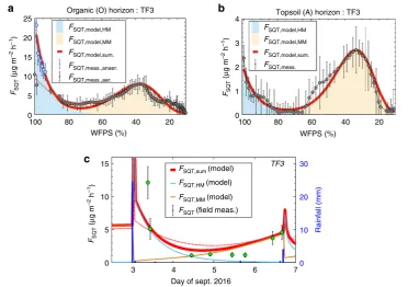
25

Organic (O) horizon : TF3

FSQT,model,HM

FSQT,model,MM

FSQT,model,sum.

FSQT,model,HM

FSQT,model,MM

FSQT,model,sum.

FSQT,sum (model)

FSQT,HM (model)

FSQT,MM (model)

FSQT (field meas.)

FSQT,meas.,anaer.

FSQT,meas.,aer.

FSQT,meas.

Topsoil (A) horizon : TF3 4

3

2

1

0 20

15

10

5

0

15

10

5

0

3 4 5 6 7

Day of sept. 2016

100 80 60 40 20

WFPS (%)

100 80 60 40 20

WFPS (%)

30

Rainfall (mm)

20

10

0

TF3

a

b

c

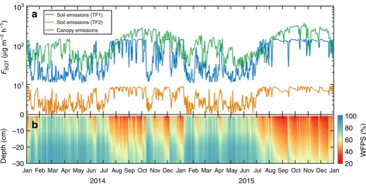
[image:5.595.114.487.305.567.2]

which (2015) was impacted by El Niño conditions. Thus, seasonal

and climatic variation of both sources could be examined. Both

soil and canopy emissions reach a maximum during the dry

season. Remarkably, soil emissions from TF1 are closely

com-parable to the tree canopy emissions, even exceeding them during

the transition from wet to dry season.

Forest canopy model

. The average dry season SQT emissions

from TF soils (44.9

μ

g m

−2

h

−1

considering emissions from TF1,

TF2, TF3, and TF4) were incorporated into a simple forest

canopy column model

34

(FORCAsT (forest canopy atmosphere

transfer)) in order to evaluate the signi

fi

cance of soil SQTs to air

chemistry. The majority of these highly reactive species were lost

through ozonolysis within the canopy space, with a maximum of

1.5% of soil emissions escaping the canopy just before dawn when

photochemistry commences and around 0.2% through most of

the day as reaction rates reach a maximum. Soil emissions of

SQTs account for as much as 50% of O

3

reactivity (soon after

dawn) at the soil surface and a relatively constant 30% during

daylight hours. Overnight, soil SQTs contribute nearly 40% of O

3

reactivity at the top of the canopy, but this is substantially

reduced to 0.5

–

1% during daylight hours as the SQTs are rapidly

consumed within the canopy. The high reactivity of SQTs results

in substantial enhancements in the concentrations of condensable

reaction products that will partition into the aerosol phase and

potentially act as cloud condensation nuclei. SQT-derived

oxi-dation products increase the total concentration of condensable

species at the top of the canopy by 30

–

40% at night when reaction

rates are low for other emitted compounds decreasing to around

20% at dusk when the contribution from other species is highest.

Discussion

Strong SQT emissions from Amazonian soils have been

quanti-fi

ed from laboratory investigations. A reproducible emission

pattern as a function of WFPS was recognized and an empirical

emission algorithm was created assuming different microbial

processes under two different moisture regimes (high moisture/

initial burst HM and medium moisture/drying out MM).

The algorithm was developed based on desiccation experiments

from sieved soils. While this approach allows the quanti

fi

cation of

purely soil-emitted VOCs, plant

–

microbe interactions, and the

possible role of an intact web on soil emissions is not addressed

here. Other soil organisms (such as fungi, roots, micro, and

macro fauna) may in

fl

uence the net effect of SQT emissions from

soils in neotropical forests and it remains to be tested how the

algorithm, evaluated with one in situ measurement period, will

perform under the seasonal changes of soil composition,

micro-biome community, and plant developmental stages. Nonetheless,

the emission pattern and strength forecasted at Fig.

5

c indicates

that laboratory incubations can be used as proxy for emissions in

the

fi

eld.

Our samples were fumigated with VOC mixing ratios at levels

that have been previously measured in the

fi

eld, although due to

experimental limitations, SQTs were not introduced in the

headspace of the chambers. Assuming a compensation point

between ingoing air and within soil SQT concentrations, the

creation of atypical concentration gradients could possibly

increase the net emission rate. Apart from the physical processes,

biological in

fl

uences may add to the uncertainties. Shown in

Fig.

4

, the samples S13 and S14 of TF5 (also S16 and S17 of TF6)

were analyzed with different experimental setups (Exp.Set.1 and

Exp.Set.2, respectively (see Methods for details)). The emission

rates display the same behavior, and the emission rate differences,

usually within the error bars, can be primarily attributed to

inter-sample variability. Another possible reason could be the absence

of VOCs in the main ingoing airstream of S13. In Exp.Set.2 we

did not fumigate and therefore the lower production of SQTs

observed (compared to S14; Exp.Set.1) could potentially indicate

a connection between ambient-other than SQT-VOCs and

microbial production in both regimes.

The initial emission burst of SQTs observed at the beginning of

each experiment (HM regime) has been variously ascribed

35

to

hypo-osmotic stress response of the soil microbes, the

replace-ment of headspace air by water and its release back to the

atmosphere and activation of rapid, intermediate, and/or delayed

responding soil microbes

36

. Chemical speciation of SQT emission

rates obtained in the

fi

eld during September 2016 (TF3) showed

distinctly different SQT species were emitted 6 h after a strong

rainfall event compared to the following dry days, showing that

different (and possibly multiple) processes are responsible for the

SQT emission bursts following rainfall. Fungal emissions are

exceptionally strong during their initial growing phase

30

and may

re

fl

ect the highest SQT species diversity and strongest

dis-crepancy between simulated and measured emissions that has

103

Soil emissions (TF1) Soil emissions (TF2) Canopy emissions

102

101 0

–10

100

WFPS (%)

80

60 40

20 –20

–30

Jan Feb Mar Apr May Jun Jul Aug Sep Oct Nov Dec JanFeb Mar Apr May Jun Jul Aug Sep Oct Nov DecJan

2014 2015

Depth (cm)

FSQT

(

μ

g m

–2

h

–1

)

a

b

[image:6.595.117.480.50.235.2]

been observed directly after the rainfall. The SQT emissions may

therefore be even stronger in seasons and regions with rapid

fungal growth rates.

Under the MM regime, SQTs displayed optimum emissions at

certain WFPS reproducibly, thus indicating the most favorable

conditions of microbially produced SQTs. The monitoring of

16S- and 18S rRNA transcripts was undertaken as a practical

means to study microbial community responses to environmental

variables

35,37

. While some taxa do not demonstrate a linear

correlation between rRNA abundance and microbial activity

38

,

ribosomes indicating potential cell activity in a community are

more abundant than in dormant cells

39

. At the community level,

an increase in rRNA content is assumed to re

fl

ect greater protein

production over time, and therefore a proxy for activity. Our

experiments demonstrated a variation of transcript abundance

between two ecologically diverse soils, and in addition, they

showed a peak of transcription coincident with SQT peak

emis-sions in the MM regime. This strongly suggests that microbial

activity inferred from ribosomal RNA can be associated with SQT

production and release.

Emission rates from two TF soils, simulated over the course of

2 years, indicated stronger emissions during the dry season when

prevailing conditions led to the WFPS associated with optimum

emissions. During the El Niño year of 2015, extended drought

conditions led to a slight decrease of SQT emission rates, as the

fi

eld WFPS dropped to about 25

–

30% for the organic (O)

hor-izon. Nonetheless, this falls within the uncertainty limits for the

optimum WFPS observed in the laboratory and the direct

implications of extended drought to microbial activity and

sub-sequent SQT release requires further investigation. The emission

strength, however, was validated with

fi

eld measurements for

both TF3 (ATTO site) and the strongest emitter TF1. The

com-parison with an established emission algorithm for vegetation

(MEGAN) indicated that soil SQT emissions from TF1 are of

comparable magnitude and so could rival the canopy emissions at

the same location under certain conditions. The inherent

uncertainties included in this comparison primarily originate

from the temperature dependency (

β

-factor) that is used for

vegetation emissions, and the large variability that has been

observed for the soil emissions. To the best of our knowledge, no

studies have directly addressed and determined the temperature

dependency of SQT emissions from Amazonian vegetation.

Hence, the present implicit assumption of a common and stable

season independent

β

-factor

=

0.17 (as used in MEGAN for all

SQT species) can be considered a

fi

rst approximation with

large-associated uncertainty as it has been shown that the

β

-factor can

vary signi

fi

cantly day to day, and with atmospheric conditions

9

.

In addition to canopy model uncertainties, soil emissions

dis-played signi

fi

cant variation in strength between the sites

investi-gated, with emission estimates ranging from a few

μ

g m

−2

h

−1

to

orders of magnitude higher. In general, soil emissions seem to be

primarily location and microbial activity speci

fi

c, as demonstrated

by TF4 and TF5.

The average dry season SQT emissions from Terra Firme soils

were incorporated into a simple forest canopy column model

33

.

The results indicated that soil SQTs dominate the ozone reactivity

close to the forest

fl

oor. Soil emissions from TF1 alone could

account as much as 75% of O

3

reactivity (soon after dawn) close

to the soil surface and have a relatively constant contribution of

50% during daytime. While a small fraction of these emissions

can escape the canopy, their oxidation products will be

con-siderable at the canopy top. The model thus suggests that not only

do emissions of SQTs from Terra Firme soils substantially affect

atmospheric chemistry within the canopy, but that the effects

have the potential to alter regional chemistry, clouds, and hence

climate.

The implications of strong soil

–

atmosphere SQT

fl

uxes from

tropical forest soils are considerable. Ecosystem emission

fl

uxes of

SQTs and their reaction products to the atmosphere above the

forest could be much larger than the currently considered canopy

source, which could contribute a part of the large reported

missing OH reactivity

40

. Beneath the canopy, the soil SQTs react

rapidly with downward-mixed ozone, impacting the oxidative

capacity within the forest

41

. Chemical reaction with soil SQT

emissions could dominate O

3

reactivity. Furthermore, any

organic particles that are formed via SQT-ozone reactions have

the potential to grow to become effective cloud condensation

nuclei

5,42

. Hence a connection between soil microbial activity,

rainfall, SQT emissions, and clouds is postulated. We consider

SQT emissions at the soil

–

atmosphere interface to be an

impor-tant unaccounted biogeochemical process that connects microbial

emissions to atmospheric chemistry and physics.

Methods

Soil characterization. Soil sampling followed a standard protocol21_{. The soil types} were characterized by using the world reference bases for soil resources43_{. Soil} samples were collected from pits of 2 m depth, dug at the vicinity of the ATTO site (for specific locations, see Supplementary Table1). Exchangeable cations and sum of base cations were determined using the silver-thiourea method44_{(cmol kg}−1_),

with elemental concentrations measured by atomic absorption spectroscopy (AAS) calibrated using suitable reference materials and blanks. For each soil, weathering conditions were determined using a total reserve bases weathering index (ΣRB).

This index takes into account the total cation concentration in the soil extractable by strong acid (H2SO4) and H2O2digestion and adding this to the reservoir of

exchangeable cations. Soil clay content was determined using the pipette method45_. The quality indexΠ21_{is a semi-quantitative soil physical quality index that adds up}

scores of four soil physical properties (effective depth, soil structure, topography, and anoxia), which influence soil morphological characteristics related to pedo-genesis. Higher values indicate less aeriated soil conditions and more frequent anoxia.

Experimental setup. A dynamic laboratory incubation system allowing automated measurement of 38 samples was used to investigate the release and uptake rates of VOCs from soil. In addition, four samples were measured with a slightly different setup that is described below (see Supplementary Table1for an overview of all 42 samples). The chamber system that was used for the majority of the samples is described in detail elsewhere22. Briefly, thisflow-through system allows control of soil temperature and atmospheric conditions (composition (e.g., VOC mixing ratio, O2content, and relative humidity)), and allows calculation of moisture content by

tracking the evaporationflux (the difference in relative humidity between inlet and outlet air) from soil46,47. In a standardized incubation procedure, 80 g of sieved (2 mm mesh)field moisture and root-free soil was wetted to saturation and tem-peratures were held constant at either 20 °C or 30 °C under VOC-free air (i.e., normal atmospheric O2concentration) and nitrogen-pressurized gas standard (i.e.,

O2and VOC-free air) (6.0, Westfahlen AG, Germany). The presence of roots in the

samples analyzed may induce unnatural emissions that originate from the rhizo-sphere and would lead to difficulties in separating soil and root emissions. Therefore, allfine roots were carefully removed from the samples, prior to their analysis. Potential remainingfine roots may increase the PTR-MS signal but their potential abundance (<0.1%) is not expected to induce the release of VOCs in a substantial manner.

The VOC-free air was produced from a zero air generator (PAG 003, Ecophysics, Switzerland), which is free of particles, and low in water (−30 °C dew point), NOx, SO2, O3, and CO. Six soil incubation chambers (Teflon foil coated,

For simultaneous quantification of gas uptake and production rates, we used a VOC calibration gas standard (14 components; Apel-Riemer Environmental, USA, diluted to the 0.1–1 ppb range) diluted with the zero air (or N2)flow. Depending

on the experiment, low and atmospherically relevant VOC mixing ratios (0.1–1 ppb) were introduced to the main airstream of VOC-free air. In addition to VOCs, CO2was constantly introduced in the main airstream. The soils were fumigated

withfield-relevant (measured) CO2mixing ratios (0–5 cm: 400–3000 ppm, 10–50

cm: 1000–14,000 ppm) during the drying out process. A custom-made electronic control system (V25, Max Planck Institute for Chemistry) was used to regulate the introduced mixing ratios for every measuring cycle. The air from the outflow of each chamber was monitored by the PTR-MS. Each chamber was monitored for 10–15 min before switching to the next chamber.

The airstreamflows were regulated by massflow controllers (Bronkhorst, Wagner Mess- und Regeltechnik GmbH, Germany), which were calibrated by a primary airflow calibrator (Gillan Gilibrator 2, Sensidyne, USA). A total of 5 l/min

flow was split into two streams. During sampling, 2.5 l/min were directed through the measuring chamber. The chambers that were not actively being sampled were continuouslyflushed with 0.5 l/min in order to continue the drying process (though at slower rates). The outlet of all chambers was connected to a single line to which the proton transfer reaction–mass spectrometer (PTR-MS) and an ultraportable greenhouse gas analyzer (Los Gattos Research Inc., USA) that measured water vapor and CO2were connected.

Experiments S3, S4, S13, and S16 were conducted with a different experimental setup (hereafter called EXPSET2) that uses the same operating principle. The same standardized procedure and soil handling was followed. The difference with the previously described system is that instead of zero air generator, synthetic air (6.0, Westfahlen AG, Germany) was used as zero air and the chambers were made from 100% Teflon (inner diameter=10 cm; chamber volume=500 ml). The same chambers were used for the determination of the emission rates in thefield (see “Flux measurements”in thefield below). In total, three main air streams (each 1 l/ m of VOC-free air) were split into two individual streams each of 0.5 l/m. In total, six chambers were operated. For these experiments, each main airstream was having a separate zero chamber that was used for the determination of background signal. The outlet of all chambers was connected to a single line to which the proton transfer reaction–mass spectrometer (PTR-MS) was connected.

PTR-MS measurements. Mixing ratios of VOCs were quantified on-line using a high-sensitivity PTR-MS (IONICON Analytik GmbH, Austria). Molecules (R) with higher proton affinity than water (691 kJ/mol) were ionized inside a low-pressure (2.2 mbar) drift tube with hydronium ions (H3O+) produced in the ion source via

electrical discharge of water vapor. The electricalfield in the drift tube accelerates the ionized molecules that arefinally detected by a quadrupole mass spectrometer at their protonated molecular mass (RH+). A detailed description of the operating principle can be found elsewhere48.

The PTR-MS was operated under standard conditions (E/N=117 Td, 600 V, 2–2.2 mbar). Humidity-dependent calibrations were performed by use of a calibration gas standard (Apel and Riemer Environmental, USA) containing methanol, acetonitrile, acetaldehyde, acetone, dimethyl sulfide, isoprene, methyl vinyl ketone, methyl ethyl ketone, benzene, toluene, o-xylene, and a-pinene. The mixing ratios of the molecules that were not present in the calibration gas (e.g., SQT) were calculated with the use of an experimentally derived transmission curve (i.e., while calibrations were used for the species in the calibration standard, SQTs were calculated by applying the instrument’s transmission curve which is a commonly used procedure for species without stable calibration sources. The transmission curve takes into account the changes in ion transmission efficiency through the detector which change with size.). The background signal was determined with VOC-free air, generated from a catalytic converter (Platinum pellets, 400 °C).

SQT ions were detected atm/z205. The reaction of SQT with H3O+

under typical drift tube conditions results in multiple fragments due to both dissociative and non-dissociative proton transfer. Therefore, detection efficiency is lower than more robust VOCs. Despite the high correlation (R2> 0.9) with the major fragment ion (m/z149), only the parent ion (m/z205) was used for the calculation of the mixing ratios. The relative abundance was derived from literature (30%)9,49, together with the reaction rate constant (kSQT+H3O+=3 × 10−9 molecule cm3_s−1₎9,50,51_{. The fragmentation pattern of SQT inside the drift} tube depends on both E/N ratio and the structure of the molecule52. The fragmentation of the dominant SQT species newly identified in this study (i.e.,

α-gurjunene,α-himacalene, andβ-eudesmene) has not previously been characterized. Hence, larger uncertainties are expected in thefinal calculation of SQT mixing ratios (≈50%).

Experiments S3, S4, S13, S14, S15, and S16 were conducted with a different but same model quadrupole PTR-MS system (hereafter referred as PTR-MS2; IONICON Analytik GmbH, Austria) that was tuned for the same drift tube conditions (E/N= 117 Td, 600 V, 2–2.2 mbar). The transmission efficiency for PTR-MS2 was lower for sesquiterpenes (TSQT,PTR-MS1=0.3,TSQT,PTRMS2=0.19) and therefore decreased

precision (Pres.PTR-MS1=9.4 ± 3.1%; Pres.PTR-MS2=15.9 ± 4.4%) was observed.

Shown in Fig.4, the samples S13, S16, and S14, S15 were analyzed with EXPSET1 and EXPSET2, respectively (using PTR-MS2). The emission rates display the same behavior and the emission rate differences (usually within the error bars) can be primarily attributed to inter-sample variability. Another possible reason

could be absence of VOCs in the main airstream of S13. In EXPSET2, we did not fumigate with environmentally relevant VOCs, therefore the lower production of SQTs observed (compared to S14; EXPSET1) could potentially indicate a connection between ambient VOCs and microbial production and future studies shall focus in identification of possible microbial mechanisms and pathways.

GC-MS measurements. Since the PTR-MS is unable to separate SQTs into individual species, additional GC-MS analysis was vital for the identification of the individual SQT structures and direct comparison of the measured emission rates (Supplementary Fig.1). Adsorbent tube samplesfilled with Quartz wool/Tenax TA/Carbograph 5TD (Markes Environmental) were used to collect air samples in parallel to the on-line measurements and these were subsequently analyzed off-line. The adsorbent tube samples were analyzed using a thermal desorption instrument (Perkin-Elmer TurboMatrix 650, Waltham, USA) attached to a gas-chromatograph (Perkin-Elmer Clarus 600, Waltham, USA) with DB-5MS (60 m, 0.25 mm, 1 µm) column and a mass selective detector (Perkin-Elmer Clarus 600T, Waltham, USA). The sample tubes were desorbed at 300 °C for 5 min, cryofocused in a Tenax TA cold trap (−30 °C) prior to injecting the sample into the column by rapidly heating the cold trap (40 °C min−1_{) to 300 °C. Afive-point calibration was performed using}

liquid standards in methanol solutions. Standard solutions (5 µl) were injected onto adsorbent tubes and thenflushed with helium (80–100 ml min−1) for 10 min to remove the methanol. The following SQTs were included in the calibration solu-tions: longicyclene, iso-longifolene,α-gurgunene,β-caryophyllene, aromadendrene, andα-humulene. Unknown sesquiterpenes were tentatively identified based on the comparison of the mass spectra and retention indexes (RIs) with NIST mass spectra library (NIST/EPA/NIH Mass Spectral Library, version 2.0). RIs were calculated for all SQTs using RIs of known SQTs and monoterpenes as reference. These tentatively identified SQTs were quantified using response factors of cali-brated SQTs having the closest mass spectra resemblance.

Calculation of release and uptake rates. The release and uptake rates of the investigated VOCs were calculated using the following equation:

FVOC¼Q

ðCoutCinÞ

A ð1Þ

WhereQis the gasflow rate through the measured chamber (in m3h−1),Coutand Cinare the VOC concentrations in the air exiting chambers holding soil samples

(soil) and empty chambers without soil (reference chamber), respectively (inμg m −3_{) andAis the headspace area of each chamber (m}2_{). Thefinal release and uptake}

rates were calculated inμg m−2_h−1_.C

outandCinwere calculated from the average

of the last four data points before the chamber switch.

Calculation of water-filled pore space. The mass of soil was determined grav-imetrically at the beginning (t0) and end (ts) of the experiment asmsoil(t0) andmsoil

(ts). Over the course of the drying out for each experiment, the shape of the H2O

signal over incubation time was converted into mass of wet soil by the use of the H2O vapor mass balance of the dynamic chamber which was further developed as a

recursion formula22as shown below:

msoilð Þ ¼ti msoilð Þ þt0 g sH2O;chamð Þ ðti VþQti2ti1Þ

sH2O;chamðti1Þ ðVþQti2ti1Þ

Qtiti1

2 ðsH2O;refð Þ þti sH2O;refðti1ÞÞ

ð2Þ

whereVis the volume of the headspace of the chamber,Qtheflow ratetiandti-1

the incubation time in seconds, andsH2O,cham(ti),sH2O,cham(ti−1),sH2O,ref(ti), and

sH2O,ref(ti-1) is the H2O signal in the soil chamber and reference chamber measured

by the ultraportable greenhouse gas analyzer (Los Gattos Research, USA) attiandti

−1, respectively. The factorgwas calculated as:

g¼ msoilð Þ ts msoilðt0Þ

Vhs_H2O;chamð Þ t_s s_H2O;chamð Þt₀iþS₀ ð3Þ

wheresH2O,cham(ts) andsH2O,cham(t0) is the signal of H2O in the soil chamber atts andt0, respectively. AndS0was calculated as:

S0¼Q

Xi¼n

i¼1ð titi1

2 þ

ti1ti2

2 Þ sH2O;chamðti1Þ sH2O;refðti1Þ

" #

ð4Þ

The mass of soil was converted into water-filled pore space [%], WFPSlabby

WFPSlabð Þ ¼ti

msoilð Þ ti msoilðtsÞ

msoilðtsÞ 100

θs ð5Þ

whereθsis the saturated gravimetric water content in the laboratory at the

soil sample (sieved through a 2 mm mesh) followed by the addition of H2O until

the surface of particles was covered by a tinyfilm of water.

Emission model. For a given temperature, our algorithm for modeling SQTfluxes incorporates the emission equation as a function of WFPS that has been developed previously for NO24_{, with the addition of a term that describes the exponential} decay of the emission burst upon wetting.

FSQTðWFPSÞ ¼aWFPSbexpðcWFPSÞ þdexpðfWFPSÞ ð6Þ

The parametersa,b,c,dandfwere related to the observed values:

a¼ FSQTðWFPSoptÞ WFPSb

optexpðbÞ

ð7Þ

b¼

ln FSQTðWFPSoptÞ FSQTðWFPSuppÞ

ln WFPSopt

WFPSupp

þWFPSupp

WFPSopt1

ð8Þ

c¼_WFPSb

opt ð

9Þ

Here,FSQTis the moisture-dependent emission,F(WFPSopt) is the highest emission

which is observed at WFPSoptandF(WFPSupp) is the emission at half maximum,

when WFPSupp> WFPSopt. The constantsdandfwere empirically derived by an

exponentialfit over thefirst 6 h after the initial wetting.

Flux measurements in the_field. Flux measurements at TF3 (ATTO is the Amazonian Tall Tower Observatory, located about 150 km northeast of Manaus, Brazil; seehttp://www.mpic.de/en/research/collaborative-projects/atto.html) and at TF1 were quantified with the use of custom-made, non-transparent Teflon chambers (inner diameter=10 cm; chamber volume=500 ml; same chambers as EXPSET2) and application of Eq. (1). On the top of each chamber were two ports that were used for the ingoing and outgoing airstream. The chambers were placed directly over litter free soil and synthetic air was pumped through the chamber with a rate of 792 ± 164 cm3_min−1_{. To avoid root damages and hence artificial}

emissions, the chambers were not installed inside a collar, but Teflon foil was used to close the surrounding of the chamber and its connection to the soil surface to achieve the minimum disturbance of the soil bellow the chamber. At the ATTO site, synthetic air from pressurized gas bottle was used for the ingoing air. Applying an activeflux though the chamber may result in an overestimation of the quantified VOCs but it will not affect the emission pattern of sampled species. Due to the remote location of some of TF1, Teflon bags werefilled with zero air prior to each experiment and connected to the inlet port before sampling. The regulation of the synthetic air inflow was made with a calibrated rotameter. A T-piece at the outlet of the chamber was used to ensure an overflow while an adsorbent tube (filled with Quartz wool/Tenax TA/Carbograph 5TD; Markes Environmental) was sampled. A total volume of 2.5–3.5 l was collected at a samplingflow rate of 167 ± 8 cm3_min−1_.

To account forflux variability due to possible soil heterogeneities, three separate samples were simultaneously (0.5–1 h difference) taken from areas in the vicinity of the pit. We note that the experiments were set up directly after the rain event (Fig.5c) and hence the soil was not covered during when rainfall occurred.

Assuming a compensation point between ambient air and within soil SQT concentrations, the use of zero air used for the ingoing air, could potentially lead to an overestimation of thefluxes measured. Nonetheless, the emission pattern forecasted at Fig.5c indicates that despitefield experimental restrictions, laboratory incubations can be used as proxy for emissions in thefield.

Upon collection, the adsorbent tubes were shipped to Finland and analyzed between 3–4 weeks later with the aforementioned method. Due to the discovery of the high abundance ofα-gurjunene in the laboratory experiments, the GC-MS quantification method for thefield measurements was performed with an authentic liquid standard.

The error propagation for the presented points has been calculated as follows:

ErF_SQT¼qffiffiffiffiffiffiffiffiffiffiffiffiffiffiffiffiffiffiffiffiffiffiffiffiffiffiffiffiffiffiffiffiffiffiffiffiffiffiffiffiffiffiffiErQ2_þErGC2_þStd2 ð10Þ

where ErFSQTis the total error for each point, ErQ is the uncertainty over the

samplingflows, ErGC is the uncertainty due to quantification of SQT, and Std is the standard deviation over the triplicates sampled at each given time. In Fig.5c all data points are the result three samples, apart from the points presented for the 3rd of September, which are the product of duplicates.

Hydrological model. One-dimensional variably saturated waterflow into soils is described by the 1D-Richards equation53:

∂θ

∂t¼

∂

∂z KðhÞ

∂h

∂zþ1

ð11Þ

whereθ_½L3_L3_{is the water content,t T½ is time,z L½ is the vertical spatial}

coor-dinate, positive upwards,h L½ is the pressure head, andKðhÞ½LT1is the unsa-turated hydraulic conductivity function.

The numerical solution of Eq. (2) requires the definition of the soil hydraulic properties (SHPs), i.e., the water retention curveθðhÞ(SWRC) and the unsaturated hydraulic conductivity curveKðhÞ(HCC). We used the van Genuchten–Mualem (VGM) model54_{for all simulations. The SWRC and HCC are given by the} equations:

θð Þ ¼h θrþðθsθrÞ 1þj jαh

n ð Þm_;h<0 θs;h0

ð12Þ

Se¼θð hÞ θr

θsθr

ð13Þ

KðSeÞ ¼KsSle 1 1S

1 m

e

m

h i2

ð14Þ

whereθsandθr½L3L3are saturated and residual water contents, respectively,

α½L1,n½ , m½ andl½ are shape parameters,m¼11

n;n>1, andSe[-] is

effective saturation.

The Richards equation was solved numerically by using the Hydrus 1D software55_{. The 1 m soil profile was divided in three different layers: upper layer} 0–10 cm, middle layer 10–20 cm, and bottom layer 20–100 cm. Each layer is described by a unique set of SHPs. A free-drainage boundary condition was used for the lower boundary (1 m) and an atmospheric boundary condition was used at the soil surface. Measured rainfall and evaporation were used as specifiedfluxes across the soil surface. The initial condition was specified as pressure head distribution given by preliminary simulations (warm up period) in order to reflect realistic conditions.

The model was calibrated againstfield measured water content values at 10, 20, and 100 cm depth. The objective function to be minimized for determining the vector of unknown parameters~p(the SHPs for the three layers) is given by the weighted-least-squares formulation

Oð Þ ¼p X N

i¼1

wiriðpÞ2 ð15Þ

whereNis the number of data points in the objective function,riare the residuals, i.e., the differences between the observed and the model-predicted data, andw_iare weights which reflect the reliability of the individual measurements. Iterative minimization of Eq. (15) with respect to the parameter vector~pwas achieved with the SCE–UA global search scheme56_{. Water content and WFPS at each depth was} calculated by conducting forward simulations with the calibrated model.

Global model of treetop emissions. The EMAC (ECHAM5/MESSy Atmospheric Chemistry) model has been used to estimate plant emissions of SQTs in the location of the ATTO tower during the years 2014 and 2015. The EMAC model is based on the 5th generation European Center Hamburg general circulation model (ECHAM557_{) and the Modular Earth Submodel System (MESSy}58_{). In the present} study, we applied EMAC (ECHAM5 version 5.3.02, MESSy version 2.52) in the T106L31-resolution, i.e., with a spherical truncation of T106, corresponding to a quadratic Gaussian grid of ~1.1 by 1.1 degrees in latitude and longitude, with 31 vertical hybrid pressure levels up to 10 hPa. The model dynamics have been weakly nudged toward ERA-Interim data59. In this study, the model was run without photochemical calculations, thus merely as general circulation model (GCM) to represent emissionfluxes. In addition, the submodel SCOUT (Stationary Column OUTput) to extract data at the location of the ATTO tower, and the MEGAN submodel were applied. The latter submodel is the implementation of the MEGAN model (Model of Emissions of Gases and Aerosols from Nature, version 2.0460₎ into EMAC, where input from the GCM is used to estimate biogenic emissions of tracers61,62. The model was run for 2 years (2014–2015) and the emissions at the location of the ATTO tower estimated by MEGAN were outputted at 1-hourly frequency via the SCOUT submodel. The SQT emissions were integrated to esti-mate the total source calculated by MEGAN in this location.

Molecular analysis. Subsamples of TF4 and TF5 soil were collected from the chambers during the desiccation experiment. Soil was sampled at moments chosen due to sesquiterpene emission profile: after wetting, after 18 h and 48 h approxi-mately, representing ESQTmaxand ESQTminvalues. Subsamples were collected

scheme was designed to provide composite pseudo-replicate samples representing the community present in the chamber at each moment. Half of the soil in each sample was used to calculate gravimetric moisture and the other half for RNA extraction. RNA was extracted with a total RNA Isolation Kit (RNA PowerSoil®, MO BIO Laboratories Inc., USA). Qubit 3.0fluorometer®(Invitrogen, USA) was used to assess RNA quantity with respective assay HS kits. An aliquot of RNA was reverse transcribed to cDNA using SuperScript®VILOTM Master Mix (Invitrogen, Karlsruhe, Germany) after DNAse treatment (DNase Max, MoBIO, CA, USA). Quantification of bacterial and fungal 16S and 18S transcript abundances per gram dry soil was performed in a StepOnePlusTM real-time PCR System (Applied Biosystems, USA). Standard curves were obtained using tenfold serial dilutions from calculated 1011 copies µl−1and 1010 copies µl−1of 16S rRNA and ITS genes, respectively, obtained from Escherichia coli (DSM 30083 strain) and Sacharomyces cerevisiae (DSM 70449 strain) genomes. We applied the primers 338F/534R for 16S rRNA and FR1/FF390 for 18S rRNA, which have been used in previous studies63,64_{. Each reaction had afinal volume of 20 µl containing 1× Power SYBR} Green PCR MasterMix (Invitrogen, Karlsruhe, Germany), 0.2 µM of each primer, and 2 µl of cDNA twofold diluted. Bacterial and fungal transcripts were amplified according to the cycling conditions: 15 min at 95 °C, followed by 40 cycles of 30 s at 94 °C, 30 s at 53 °C (50 °C for the fungal primers) and 30 s at 72 °C (1 min of extension for the fungal primers). SYBR greenfluorescence was measured after the elongation step for each run. TheR2and the efficiency of amplification were 0.998 and 89.9 and 0.994 and 86.2 for bacterial and fungal standard curves, respectively. Each gene was assayed for all samples in two separate runs with duplicates for each sample, withfinal four replicates standardized between runs.

Canopy model. The FORCAsT (FORest Canopy Atmosphere Transfer) model34 has been used to simulate soil emissions and processing of SQTs within the rainforest canopy. The model was run over 48 h for an average meteorology for September 2014, derived from in situ observations at the ATTO site, and the output of thefirst day discarded as spin-up. Initial concentrations of biogenic VOCs, ozone, NOx, CO, and CO2within and just above the canopy were taken

from observations made during this and previous measurement campaigns at this site27,65,66. The average height of the canopy was taken to be 40 m and it was assumed that the forest around the site was homogeneous. Soil characteristics were taken from Andreae et al.27_{and vertical distribution of leaf area was based on Kuhn} et al.67.

SQTs were introduced into the model at the soil–atmosphere interface at a constant rate of 44.9μg m−2_h−1_{, representing the average emissionflux measured}

from Terra Firme soils in the dry season. 10% of the emitted SQTs were assumed to beβ-caryophyllene and the remainder lumped as“other SQTs”.β-caryophyllene chemistry follows the master chemical mechanism for thefirst two generations of oxidation products with subsequent products lumped; only the initial reactions of

“other SQTs”(with O3, and the OH and NO3radicals) are explicitly included.

FORCAsT does not include an aerosol phase but does explicitly calculate the rate of formation of low volatility oxidation products, which are assumed to condense into particles34.

Data availability. The data sets within the article and Supplementary Information of the current study are available from the authors on request.

Received: 4 September 2017 Accepted: 15 May 2018

References

1. Gershenzon, J. & Dudareva, N. The function of terpene natural products in the natural world.Nat. Chem. Biol.3, 408–414 (2007).

2. Schmidt, R., Cordovez, V., de Boer, W., Raaijmakers, J. & Garbeva, P. Volatile affairs in microbial interactions.ISME J.9, 2329–2335 (2015).

3. Peñuelas, J. & Staudt, M. BVOCs and global change.Trends Plant Sci.15, 133–144 (2010).

4. Riipinen, I. et al. The contribution of organics to atmospheric nanoparticle growth.Nat. Geosci.5, 453–458 (2012).

5. Bonn, B. & Moortgat, G. K. Sesquiterpene ozonolysis: origin of atmospheric new particle formation from biogenic hydrocarbons.Geophys. Res. Lett.30, https://doi.org/10.1029/2003GL017000(2003).

6. Vickers, C. E., Gershenzon, J., Lerdau, M. T. & Loreto, F. A unified mechanism of action for volatile isoprenoids in plant abiotic stress.Nat. Chem. Biol.5, 283–291 (2009).

7. Staudt, M., Bourgeois, I., Al Halabi, R., Song, W. & Williams, J. New insights into the parametrization of temperature and light responses of mono - and sesquiterpene emissions from Aleppo pine and rosemary.Atmos. Environ.

152, 212–221 (2017).

8. Duhl, T. R., Helmig, D. & Guenther, A. Sesquiterpene emissions from vegetation: a review.Biogeoscience5, 761–777 (2008).

9. Bourtsoukidis, E. et al. Ozone stress as a driving force of sesquiterpene emissions: a suggested parameterisation.Biogeoscience9, 4337–4352 (2012). 10. Farré-Armengol, G. et al. Ozone degradesfloral scent and reduces pollinator

attraction toflowers.New Phytol.209, 152–160 (2016).

11. Kesselmeier, J. & Staudt, M. Biogenic volatile organic compounds (VOC): an overview on emission, physiology and ecology.J. Atmos. Chem.33, 23–88 (1999).

12. Pollmann, J., Ortega, J. & Helmig, D. Analysis of atmospheric sesquiterpenes: sampling losses and mitigation of ozone interferences.Environ. Sci. Technol.

39, 9620–9629 (2005).

13. Sindelarova, K. et al. Global data set of biogenic VOC emissions calculated by the MEGAN model over the last 30 years.Atmos. Chem. Phys.14, 9317–9341 (2014).

14. Acosta Navarro, J. C. et al. Global emissions of terpenoid VOCs from terrestrial vegetation in the last millennium.J. Geophys, Res.119, 6867–6885 (2014).

15. Horváth, E. et al. Experimental evidence for direct sesquiterpene emission from soils.J. Geophys. Res.117,https://doi.org/10.1029/2012JD017781(2012). 16. Asensio, D., Owen, S. M., Llusià, J. & Peñuelas, J. The distribution of volatile

isoprenoids in the soil horizons around Pinus halepensis trees.Soil Biol. Biochem.40, 2937–2947 (2008).

17. Aaltonen, H. et al. Boreal pine forestfloor biogenic volatile organic compound emissions peak in early summer and autumn.Agric. For. Meteor.151, 682–691 (2011).

18. Leff, J. W. & Fierer, N. Volatile organic compound (VOC) emissions from soil and litter samples.Soil Biol. Biochem.40, 1629–1636 (2008).

19. Peñuelas, J. et al. Biogenic volatile emissions from the soil.Plant Cell Environ.

37, 1866–1891 (2014).

20. Brando, P. M. et al. Abrupt increases in Amazonian tree mortality due to drought–fire interactions.PNAS111, 6347–6352 (2014).

21. Quesada, C. A. et al. Variations in chemical and physical properties of Amazon forest soils in relation to their genesis.Biogeoscience7, 1515–1541 (2010).

22. Behrendt, T. et al. Characterisation of NO production and consumption: new insights by an improved laboratory dynamic chamber technique.Biogeoscience

11, 5463–5492 (2014).

23. Oswald, R. et al. HONO emissions from soil bacteria as a major source of atmospheric reactive nitrogen.Science341, 1233–1235 (2013).

24. Meixner, F. X. & Yang, W. X. inDryland Ecohydrology(eds Paolo D’Odorico & Amilcare Porporato) 233–255 (Springer, the Netherlands, 2006). 25. Karl, T. et al. Exchange processes of volatile organic compounds above a

tropical rain forest: implications for modeling tropospheric chemistry above dense vegetation.J. Geophys. Res.109,https://doi.org/10.1029/2004JD004738 (2004).

26. Asensio, D., Peñuelas, J., Filella, I. & Llusià, J. On-line screening of soil VOCs exchange responses to moisture, temperature and root presence.Plant Soil

291, 249–261 (2007).

27. Andreae, M. O. et al. The Amazon tall tower observatory (ATTO): overview of pilot measurements on ecosystem ecology, meteorology, trace gases, and aerosols.Atmos. Chem. Phys.15, 10723–10776 (2015).

28. Doughty, C. E. et al. Drought impact on forest carbon dynamics andfluxes in Amazonia.Nature519, 78–82 (2015).

29. Blazewicz, S. J., Barnard, R. L., Daly, R. A. & Firestone, M. K. Evaluating rRNA as an indicator of microbial activity in environmental communities: limitations and uses.ISME J.7, 2061–2068 (2013).

30. Weikl, F., Ghirardo, A., Schnitzler, J. P. & Pritsch, K. Sesquiterpene emissions from Alternaria alternata and Fusarium oxysporum: effects of age, nutrient availability, and co-cultivation.Sci. Rep.6, 22152 (2016).

31. Insam, H. & Seewald, M. S. A. Volatile organic compounds (VOCs) in soils. Biol. Fert. Soils46, 199–213 (2010).

32. Rasmann, S. et al. Recruitment of entomopathogenic nematodes by insect-damaged maize roots.Nature434, 732–737 (2005).

33. Liptzin, D., Silver, W. L. & Detto, M. Temporal dynamics in soil oxygen and greenhouse gases in two humid tropical forests.Ecosystems14, 171–182 (2011).

34. Ashworth, K. et al. FORest canopy atmosphere transfer (FORCAsT) 1.0: a 1-D model of biosphere-atmosphere chemical exchange.Geosci. Model Dev.8, 3765–3784 (2015).

35. Barnard, R. L., Osborne, C. A. & Firestone, M. K. Responses of soil bacterial and fungal communities to extreme desiccation and rewetting.ISME J.7, 2229–2241 (2013).

36. Placella, S. A., Brodie, E. L. & Firestone, M. K. Rainfall-induced carbon dioxide pulses result from sequential resuscitation of phylogenetically clustered microbial groups.PNAS109, 10931–10936 (2012).

37. Klein, A. M. et al. Molecular evidence for metabolically active bacteria in the atmosphere.Front. Microbiol.7, 772 (2016).