A Fuzzy Paradigmatic Clustering
Algorithm
Farzad Amirjavid∗ Sasan Barak∗∗ Hamidreza Nemati∗∗∗
∗Edward S. Rogers, Department of Electrical and Computer
Engineering, University of Toronto, Toronto, Canada (e-mail: [email protected]).
∗∗Department of Management Science, Lancaster University
Management School, Lancaster, UK (e-mail: [email protected])
∗∗∗Engineering Department, Lancaster University, Lancaster, UK
(e-mail: [email protected])
Abstract:Clustering algorithms resume the datasets into few number of data points such as centroids or medoids, which explain the entire dataset briefly. In the domain of data-driven machine learning, the more precision with the clustering rule leads directly to more precise classification, prediction, and recognition. We propose an efficient clustering method, which applies the paradigms - mainly 3D Gaussian model - to estimate the optimum cluster number, cluster border, and congestion coordinates to model the datasets of the natural distributions. This approach considers both qualitative and quantitative features of the dataset and calculates the best scale to analyze it. We used fuzzy logic to compare the models with data, to generate and rank the hypotheses, and finally to reject or accept the assumptions. The proposed approach which is called Fuzzy Gaussian Paradigmatic Clustering (FGPC) algorithm is used as the basis of a fast (with the complexity order ofO(n)) and robust algorithm for identifying fuzzy models.
Keywords:Paradigmatic clustering, Fuzzy logic, Gaussian distribution.
1. INTRODUCTION
In the heart of data-driven modeling methodologies, there are clustering processes that cohort similar data points while avoiding grouping of the dissimilar data points. The purpose of the grouping operation is to extract natural groupings of data from a large data set and to discover the strategic data points (or coordinates on the Cartesian plane) that represent the corresponding data groups. Improvement in precision and methodology of the clustering operation leads to a better perception of a system’s behavior, more precise classification, and more confident prediction (Sun et al. (2018); Hruschka et al. (2009)).
Technically, the traditional and conventional clustering algorithms look for congestion with the datasets if drawn on the Cartesian plane (Sun et al. (2018); Hruschka et al. (2009); Bezdek (2013); Hartigan and Wong (1979); Amir-javid et al. (2014b,a)), and recommend the congestion centers as the cluster centers. However, we know two interpretations of the term congestion: our first take on the congestion is a quantitative view and refers to the distribution of the data points in particular common re-gions at the Cartesian plane. For instance, the K-means algorithm (Hartigan and Wong (1979)) finds the crowded regions and returns the congestion centers as the centroids. However, there are qualitative approaches such as Fuzzy Subtractive Clustering (FSC) (Chiu (1994)) which ignore the mentioned quantitative features but focus on distribu-tion of the data values. In this work, we are proposing a
fuzzy Gaussian paradigmatic clustering (FGPC) approach, which lets cluster estimation within complexity order of
O(n). The data of distributions are the primary target of this algorithm, and the returnee of the algorithm is a model that considers both of quantitative and qualitative features of the dataset in modeling.
FGPC escapes comparison of data points to each other, thus significantly reduces the complexity order of the mod-eling process. Alternatively, it compares the data with a basic model and explains the data with likelihood regard-ing that model; and for the particular case of the natural distributions, we are using a 3D Gaussian filter. Other than the complexity order, and attention to the qualitative and quantitative features of the dataset, we propose to consider also the resulted classification precision as the second criterion to compare the clustering algorithms. By classification accuracy, we address the confidence/strength in acceptance or rejection of the samples to the discovered models. Therefore, as the second novelty of this work, since the FGPC considers both of the quantitative and qualitative features of the data, then it proposes differ-ent coordinations rather than the returnees of the major clustering algorithms such as K-means, Fuzzy C-Means (FCM), and FSC which leads to better classification pre-cision and compatible efficiency rates.
of the model with other works. Finally, we conclude the present paper and propose suggestions to the interested researchers in section (5).
2. PROBLEM STATEMENT
By reviewing some recent works on cluster analysis and machine learning (Rouzbahman et al. (2017); Sanz et al. (2015); Vluymans et al. (2016); Bassoy et al. (2017)) it can be inferred that today the machine learning experts explore the study through building a model from sample inputs which are usually transformable to a set of IF-THEN rules. The conversion of the dataset to model is the core functionality of the clustering algorithms and classifi-cation is the basic application of the models. Convention-ally, the main traditional clustering algorithms such as K-Means, FCM, and FSC and their derivations estimate the cluster centers in forms of single points called centroids and medoids within a symmetric range of influence or cluster radius. Practically, the machine learning experts use that information in fields of prediction, trend estima-tion, pattern recogniestima-tion, and other sorts of data analytics applications.
The existing major and popular clustering algorithms such as K-means, FCM, and FSC are either purely qualitative or purely qualitative. The quantitative methodologies such as K-means focus on distribution of the data points in particular regions of the Cartesian plane and estimate the center of the congestions as the centroids. On the other hand, the qualitative approaches such as FSC focus on distribution of the data values, and they select the data point that is the most similar to the neighbor data points as the medoid. These approaches face relatively weak classification confidence/accuracy rates (Sanz et al. (2015); Vluymans et al. (2016)) for two specific reasons. The modeling with quantitative methods is fast but not efficient; since with a dataset, several congestions at closed common coordinates might occur then it leads to difficulty in separation of the data groups and consequences the imprecision with classification. Even though, the quali-tative approaches are more efficient; they face again the weak classification confidence/accuracy rate problem. It is because they ignore the weight of the regions with the higher number of data points. By comparing the data points to each other, the traditional approaches are in the order of O(n2) (Tan (2005)), which makes it very
time-consuming for modeling, classification and prediction of large datasets. In prior to begin the clustering rule, they require knowing expert configurations such as number of clusters or the influence range. They consider either the qualitative or quantitative features of the data; while, the proposal of a compromiser method could decrease the error with cluster center estimation process. In this paper, we propose a method to overcome the limitations mentioned above and improve the clustering process of natural distribution datasets regarding the classification accuracy, efficiency and complexity order.
3. MODELING THE FGPC
Let us consider the matrix dn,m indicates n of the m
[image:2.595.346.514.72.148.2]-dimensional data of the series D. The d2n,m,m is a n×
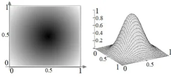
Fig. 1. 3D Gaussian curve on the Cartesian plane as the paradigm for clustering.
m×mmatrix which holds the corresponding pairs of the
xn,m:
d21:n,1:m,1:m= n Y
i=1
di,1:m×di,1:m (1)
The paradigm P is a mathematical model, which repre-sents relationships between points as of a mathematical function.
P =R(x, y)|x, y∈[0,1] (2) Therefore, a paradigm or a training model is a relationship such as a mathematical function. In this paper, by the notion PG we refer to the specific paradigm that we
compare the datasets of our experiment to a 3D curve of a Gaussian distribution.PG sits in the center of a one
by one square and its maximum height is one. See Fig.1. The equation that makes the model mentioned in Fig.1 is as of the following:
PG=Z(x, y) = 1.72×e−
(x−0.5)2 +(y−0.5)2
0.05 (3)
In equation 3, the value ofZ(x, y) indicates the quantity of the data points at the (x, y). Therefore, thePG indicates
explicitly the congestion of the matching dataset around the center of the Cartesian plane:
µCR=(0.5,0.5)= 1.72×e−
(x−0.5)2 +(y−0.5)2
0.05 (4)
By equation 4, we are indicating that the possibility degree of being the congestion center of the dataset (cluster representatives or CR) decreases smoothly with the slope ofZ0. The FGPC will model the datasets how much they respect this rule in equation 4. The paradigm of equation (3) is used to compare the datasets within variant scales. The FGPC segments the data into equal-size rectangles whileais the width, and b is the length of the rectangle.
φaandφbare the number of the segments that the FGPC
divides the rectangle edges at each step:
a= 1
φa , b= 1
φb
| φa, φb∈N (5)
Since, a and b divide the data in some steps by the rate of φ1, and they have variable values, then we refer to the value ofaandbat each step by theasandbs. By dividing
the data into equal-size rectangles, we will have a list of
a in b regions. We refer to each area by the notion As,i
orAa,b,x,y.sindicates thesegmentation strategy, andiis
the index of the segment created by that segmentation number. By the notion qs,i or qa,b,x,y we refer to the
rectangle which is q|q ∈ [0,1], q = qa,b,x,y
n . For instance,
the first row of theM is as of the following:
Ms=1=
s i a b x y q
1 1 1 1 0 0 1 (6)
In 6, s is the segmentation step, and i is the CR index.
a, b, x, y, and q indicate the coordination of the CR. By the parameter q the FGPC reflects the effect of the “local quantitative features of the dataset”, while by considering the existence of the data points in separate regions the FGPC reflects the qualitative characteristics of the data points. The datasets within different scales show different qualitative and quantitative properties leading to estimation of various congestion centers. Therefore, discovering a single invariant entity is a critical issue to model the data. For this objective, the FGPC partitions the data into smaller regions and analyzes the data of each area separately, which means it compares the data of each partition by thePG:
Dists,i=Distance(PG,[xs,i+ as
2 ;ys,i+
bs
2;qs,i]) (7) By equation 7, the FGPC measures how much the data distribution with D is alike the PG. Since there are
probably more than one CR at each segmentation step, then we propose three other parameters as the criteria of comparison:
AIDs= as×bs
P
i=1
Dists,i
n
XIDs=M ax(Dists,i)|ii==1as×bs IIDs=M in(Dists,i)|ii==1as×bs
OCEs=Average(AIDs, XIDs, IIDs)
(8)
The FGPC continues the segmentation process up to status whereas further segmentation does not lead to further congestions at around the center of the Cartesian plane but the corners:
IF (OCEs+1≥OCEs) T HEN ISE=Ms;
Stop Segmentation();
EN D IF
We call the optimum scale to model the data by invariant scale entity (ISE). This model indicates a segmentation strategy by which the data is viewed the most alike a 3D Gaussian distribution (See equation 4). In this way, the FGPC defines the dataset as a fuzzy Gaussian distribution with five parameters which are: List of Cluster Representatives (LCR), “minimum inter distance” (IID), “maximum inter distance” (XID), “average inter distance” (AID), and Overall Classification Error (OCE).
So far, we have covered the overall structure of the FGPC algorithm; however, there are more details included. Definition 1: Density of the data points (ρ).This is to specify the minimum number of data points in an area of one-by-one. The FGPC recognizes a section as equal as empty if the corresponding number of data points is smaller than ρ:
IF ( qs,i as×bs
≤ρ) T HEN
Remark Empty Zone(s, i);
EN D IF
By remarking the low-dense or empty zones, the FGPC prevents further analysis of those zones.
Theorem1:Cluster.The areaAs,i is dense ifqs,i ≥ρ. A
dense area is modeled by comparison to PG. The center
of theAs,i is the center of the zoneAj. With FGPC each
dense zone is a cluster.
Definition 2: Cluster Representative (CR). The cluster Representative of the zoneAs,i is in the following
coordinations:
CRs,i.x=xs,i+ as
2, CRs,i.y=ys,i+
bs
2 (9)
The cluster center is derived from a dense zone, else since the required congestion is not formed then further processes to calculate the cluster and cluster center would be ruled out. The circle surrounding the positionYj and Xj is the corresponding cluster:
(x−CRs,i.x)2+ (y−CRs,i.y)2= ( aj+bj
2 )
2 (10)
Definition 3: Model Fitness Parameters (M F P). This is the collection of the following parameters: XID,
IID,AID, andOCE.
Definition 4: The List of Cluster Representatives (LCR). The coordinations of the cluster representatives are in the vectorLCR. ByLCCs,i we refer to the cluster
center of the zoneAs,i. The coordinations of the items of
theLCRcome from equation (9).
Definition 5: Dataset model. The model of dataset
D is the collection of PG, LCR, and M F P including M and s as meta data. The FGPC describes the model of the dataset D in comparison to a predefined model here PG. The PG, M F P, and LCR indicates the
prop-erties of such comparison. The initial visual comparison of dataset D at the first step, is to compare it with a 3D Gaussian curve that rises in center of the Cartesian space. In equation (3) the mathematical representation and in Fig. 1, the visual representation of the Gaussian model is presented. At each step, the centroid estimation error per each coordination (xoryaxis) is maximum 0.5. Therefore, in the maximum error in centroid estimation is:
p
0.52+ 0.52 = 0.7071. Although, regardless of the data content, the initial presumption of the FGPC is a Gaussian curve formed around the (0.5,0.5). In the next step, the FGPC segments the possibilistic area into smaller zones, so that the CR estimation error decreases.
Theorem 2: Invariant Scale Entity (ISE).This is the collection of optimumM F P, and the correspondingLCR
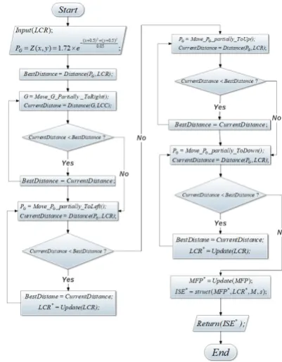
including the M and s as the meta data. For calculating the ISE, the FGPC continues segmentation of data into subsections, and matching models to data andLCRitems until the model fitness parameters (M F P) match the minimum requirements (initiated by the user), or until the matching errors do not improve (or even worsen). In other words, whenever the matching errors at steps by further segmentation increase then the segmentation and model fitting process stops. The algorithm to calculate theISE
and theM F P is in Fig.2. By the algorithm in Fig.2 the FGPC archives a sort of data segmentation that matches the most economically to a Gaussian distribution; however, the default Gaussian model (see equation (3)) might be far similar to the currentISE. TheISEis a sort of collection and the best scale to analyzeDis:ISE.s, which indicates the most economical count of clusters to modelD. Theorem 3: The optimum Invariant Scale Entity (ISE∗).To calculate a better fitting Gaussian ISE to data the FGPC moves the default Gaussian model toward both ofxandy dimensions partially. In fact, the PG might be
model fits better to the dataset. For this objective, the model is moved partially to right and left, and up and down. In this way, while the distance of the LCC members to the Gaussian model decreases then the moving act continues. Finally, the FGPC arrives at a coordination that no move from there toward any of the axes would improve the MFP. See the algorithm in Fig. 3. By the algorithm in Fig. 3, the FGPC represents its best estimation to describe data segmentations as parts of a Gaussian distribution. The LCR includes centroids, while M F P includes the reasoning criteria to inclusion of a data point to the trainee dataset.
Definition 6: Efficiency.By the criterion efficiency, we are addressing how much an algorithm is advantageous to achieve a fundamental goal of clustering, which is the maximization of the inter-cluster distances while minimiz-ing the intra-cluster distances:
Ef f iciency=
as×bs
P
k=1
as×bs
P
j=1
Distance(CRk, CRj)
as×bs
P
c=1
mc
P
i=1
Distance(ClusterM emberc,i, CRc)
, k > j (11)
In (11), themc indicates the number of clusters members
in cluster c. By the equation (11), we are indicating that theefficiency is a ratio representing the proportion of the sum of intra-cluster distances to the sum of inter-cluster distances. Obviously, if an algorithm proposes far centroids while keeping cluster members closed to each other, then we recognize it as an “efficient” approach.
4. EXPERIMENTING THE FGPC
[image:4.595.327.528.71.329.2]Efficient, precise, and fast clustering of the data points of natural distributions within complexity order of O(n) is the main subject of this experiment. For this objective, we selected analysis of the Iris dataset. It consists of the measurements of four attributes of 150 iris flowers from three types of irises’ (Setosa, Versicolour, and Virginica) petal and sepal length, stored in a 150x4 matrix. The rows of this dataset being the samples and the columns being: Sepal Length, Sepal Width, Petal Length and Petal Width. We survey the functionality of the FGPC in two stages including the qualitative functionality of the FGPC (the success in the separation of different concepts and also in the union of the similar concepts) and quantitative func-tionality (the number of times the algorithm successfully
Fig. 2. The FGPC algorithm to make ISE
Fig. 3. Fitting the Gaussian Model to centroids
classifies the Iris items).Then in the context of the single cluster center, we compare the results with other popu-lar available approaches (K-means, FCM, and subtractive clustering).
4.1 Calculation of the best scale (ISE.s) to model the Iris data
To find the ISE, the FGPC requires knowing the optimum number of clusters or the best scale (ISE.s) for modeling the dataset so it begins partitioning the data into (here equally sized) rectangles (here squares). At each step, it counts the number of data points in each partition (qs,i or qa,b,x,y) and indicates each partition by a 3D coordination.
Then FGPC compares the 3D data points with the basic paradigm (PG) to find the Euclidian distance between
the structural model and the 3D points in space. See equation (7). If the distance of the 3D points and the Gaussian model improves by further sectioning the data, then the FGPC continues the segmentation process. It stops whenever further segmentation does not economise or does not improve the distance between the 3D points and the underlying paradigm. See Fig. 2.
In this experiment, at the first step the first two columns of the Iris data are normalized using the following:
||D.x||= Iris(1 : 150,1)−min(Iris((:,1)) M ax(Iris((:,1))−min(Iris((:,1)) + 1,
||D.y||= Iris(1 : 150,2)−min(Iris((:,2)) M ax(Iris((:,2))−min(Iris((:,2)) + 1
(12)
In the next step, in order to discover theISE, the FGPC divides each axis of the dataset into equally sized i|i =
[image:4.595.87.247.582.745.2]Fig. 4. Classification error measures of FGPC basic model on Iris data
Table 1. The fuzzy centroids of the Iris data.
z represents the possibility degree to be a centroid.
Segments No. Segment index x y z Cluster radius
1 1 0.5 0.5 1 0.5
2 1 0.25 0.25 0.4067 0.25 2 2 0.25 0.75 0.2267 0.25 2 3 0.75 0.25 0.3067 0.25 2 4 0.75 0.75 0.0600 0.25
φa and φb (see equation (5)), the FGPC segmented the
data totally seven times into once 1, then 4, 9, 16, 25, 36, and finally 49 sections. The classification error measures of the clustering, which are the “Euclidean distances” between the data points and the basic Gaussian paradigm are in Fig. 4. As this is shown in Fig. 4, by beginning the segmentation from single partition to four squares, the overall classification error improves; however, by further data partitioning the OCE factor does not improve notice-ably. By continuing the data segmentation after quarterly partitioning, the worst case of error (XID) worsens, and the best case of clustering (IID) improves; however the average error rate (AID) would not necessarily improve and four segments/clusters is setted.
4.2 Iris Dataset Modeling with Single Cluster Representative
After that the optimum number of clusters is determined by the FGPC, which indicates ISE.s = 2 then it deter-mines the cluster center coordinations. The 3D coordina-tions of the centroids are in Table 1. According to the algorithm proposed in Fig. 2, the FGPC classification error rate might be improved by transiting the center of the basic paradigm from [0.5,0.5] toward left and right, and toward up and down. The 3D models, which are the data points in Table.1 give the best fitting rates (or the least total Euclidean distance) when the center of the paradigm is at [0.5,0.45]. In other words, the FGPC could find the best match of the Gaussian paradigm to the Iris data using the following:
G∗=Z∗(x, y) = 1.72×e−(x−0.5)2 +(0.05y−0.45)2 (13)
By the use of symbol ∗ we are referring to the optimum results of the FGPC rather than the primary results given in Table. 1. By the use of equation in 13, the FGPC proposes to return the coordinationC∗= [0.5,0.45] as the cluster center of the Iris data. However, since the fitting steps are in size of 0.01, then Overall error measure for this coordination is p0.12+ 0.12 = 0.14142135. By the
C∗∗ we are referring to the optimum centroid with the minimized error caused by the fitting process. Hereafter, by the F GP C∗ we are referring to the results of the FGPC those are taken by the fitting process. A comparison
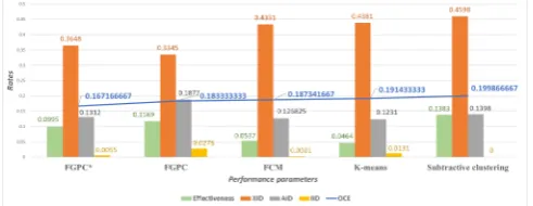
of results between FGPC, and the other popular major clustering algorithms are in Table 2. According to Table 2, the FGPC returns a different coordinations rather than the Mean, K-means, FCM and Fuzzy Subtractive Clustering (FSC) methods for the Single Cluster Center. The overall classification error rate of the FGPC is also different, because it improves coverage of the data points those are far from the cluster center. This is though the FGPC recommends to segment the data into four sections. When the number of clusters is more than one, then the problem of clustering efficiency arises. By the term “clustering efficiency” we mean to estimate cluster centers that are far from each other while it minimizes the intra-distance between the cluster members. In Fig. 5 we are showing the FGPC efficiency in clustering and precision in classification in comparison with the other approaches. By four clusters of data, in regard of inter-cluster distance factors, the FGPC gives the best classification error rates. In regard of cluster estimation efficiency the subtractive clustering algorithm gives the best rate; however, the FGPC shows better efficiency rates rather than the K-means and FCM.
4.3 Experimenting quantitative functionality of the FGPC
Applying the qualitative reasoning and according to the information in Fig. 4 the optimum number of clusters to group the first two columns of the Iris data is four. This is though in the real world the Iris data contains three classes. All 150 items of the Iris data are classified using the four clusters, once by FGPC and once by FGPC*. We call the real world classes of the Iris by “CLASS 1”, “CLASS 2”, and “CLASS 3”. In Iris, there are 50 items in each class. These are the known classes and we use them to verify how much the algorithm classifies according to the reality. We refer to assignments of the algorithm classification by “GROUP 1”, “GROUP 2”, “GROUP 3”, and “GROUP 4”. Since the number of the clusters are bigger than the number of classes, then the algorithms over-cluster the data. In other words, the FGPC identifies two groups of data points inside class of “CLASS 3”; how-ever, the algorithm which matches perfectly the real world should recognize these items within one group. Therefore, we consider the smaller rate of the over-clustering as an indicator of the better matching of the algorithm to the real world. Considering the over-clustering, then the true classification rate are in Table. 3. The FGPC* gives a lower amount of over-clustering in comparison to the other main clustering algorithms. In other words, it classified a bigger number of similar items into common groups, while it avoids better the separation of the similar objects. As
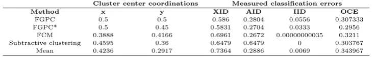
[image:5.595.309.555.639.734.2]Table 2. Comparison of the centroid estimation error measures with three major algorithms
Cluster center coordinations Measured classification errors
Method x y XID AID IID OCE
FGPC 0.5 0.5 0.586 0.2804 0.0556 0.307333 FGPC* 0.5 0.45 0.5831 0.2704 0.0333 0.2956
FCM 0.3888 0.4166 0.6961 0.2672 0.00000000035 0.3211 Subtractive clustering 0.4595 0.36 0.6479 0.6479 0 0.303767
[image:6.595.116.485.90.146.2]Mean 0.4236 0.2917 0.7364 0.2886 0.0069 0.343967
Table 3. Over-clustering of Iris data by FGPC and other major clustering approaches
Real world classes Revised true classification rate Iris real world classes CLASS 1 CLASS 2 CLASS 3
Number of items in each class 50 50 50 Number of identified subclass
items GROUP 4 by FGPC N/A N/A 15 0.68 Number of identified subclass
items GROUP 4 by FGPC* N/A N/A 11 0.7933 Number of identified subclass
items GROUP 4 by FCM N/A N/A 21 0.7733 Number of identified subclass
items GROUP 4 by FSC N/A 12 N/A 0.76
a result, the FGPC* identified more precisely the natural groupings within the data of natural distributions of the Iris data, which is the consequence of the efficient and precise clustering of the data within the modeling process.
5. CONCLUSION AND FUTURE WORKS
The proposed FGPC method segments the datasets of the natural distributions into sections until a Gaussian distribution of the data points’ quantities and their values is found. That particular segmentation is an invariant scale model, which represents the best scale to analyze the dataset and best number of clusters for centroid esti-mation. The main problem that the FGPC deals with is consideration of both qualitative and quantitative features of the data in clustering process. In overall, we recognize the FGPC standing between the purely qualitative and purely qualitative methods. In comparison with quanti-tative approaches, it gives better efficiency rates, while compared to qualitative methods it provides better classi-fication error rates.Although the existing major clustering methods require basic configuration (expert idea) to es-timate the number of clusters and the cluster size, the FGPC method estimates this parameter by complexity order ofO(1).This would help to design the more precise predictors, that act as fast as of complexity order ofO(n). The proposed paradigmatic clustering method targets the data of natural distributions; however, by considering dif-ferent paradigms we will propose further efficient and high-performing methodologies for data-mining.
6. ACKNOWLEDGMENT
We are deeply thankful to Konstantinos N. Plataniotis ([email protected]) for the constructive comments. The second author is supported by the Czech Science Foundation (GACR Project GA 18-15530S). The third author’s work is supported by the Engineering and Phys-ical Sciences Research Council (EPSRC), grant number EP/R02572X/1, and the National Centre for Nuclear Robotics (NCNR).
REFERENCES
Amirjavid, F., Bouzouane, A., and Bouchard, B. (2014a). Activity modeling under uncertainty by trace of objects
in smart homes.J. Ambient Intelligence and Humanized Computing, 5, 159–167.
Amirjavid, F., Bouzouane, A., and Bouchard, B. (2014b). Data driven modeling of the simultaneous activities in ambient environments. J. Ambient Intelligence and Humanized Computing, 5, 717–740.
Bassoy, S., Farooq, H., Imran, M.A., and Imran, A. (2017). Coordinated multi-point clustering schemes: A survey. IEEE Communications Surveys Tutorials, 19, 743–764. Bezdek, J.C. (2013). Pattern recognition with fuzzy objec-tive function algorithms. Springer Science and Business Media.
Chiu, S.L. (1994). Fuzzy model identification based on cluster estimation. J. Intelligent and fuzzy systems, 2, 267–278.
Hartigan, J.A. and Wong, M. (1979). Algorithm as 136: A k-means clustering algorithm. J. Royal Statistical Society, Series C (Applied Statistics), 28, 100–108. Hruschka, E.R., Campello, R., Freitas, A., et al. (2009). A
survey of evolutionary algorithms for clustering. IEEE Trans. Sys., Man, and Cyber., Part C (Applications and Reviews), 39, 133–155.
Rouzbahman, M., Jovicic, A., and Chignell, M. (2017). Can cluster-boosted regression improve prediction of death and length of stay in the icu?IEEE J. Biomedical and Health Informatics, 21, 851–858.
Sanz, J.A., Bernardo, D., Herrera, F., Bustince, H., and Hagras, H. (2015). A compact evolutionary interval-valued fuzzy rule-based classification system for the modeling and prediction of real-world financial appli-cations with imbalanced data. IEEE Trans. Fuzzy Sys-tems, 23, 973–990.
Sun, S., Wang, S., Wei, Y., and Zhang, G. (2018). A clustering-based nonlinear ensemble approach for ex-change rates forecasting. IEEE Trans. Sys., Man, and Cyber., Systems, 1–9.
Tan, P.N. (2005). Introduction to Data Mining. Pearson, USA.