An Efficient Proximal Point Algorithm for Unweighted Max Min Dispersion Problem*

(1)

http://www.scirp.org/journal/apm ISSN Online: 2160-0384

ISSN Print: 2160-0368

DOI: 10.4236/apm.2018.84022 Apr. 18, 2018 400 Advances in Pure Mathematics

An Efficient Proximal Point Algorithm for

Unweighted Max-Min Dispersion Problem

*

Siqi Tao

Department of Mathematics, College of Sciences, Shanghai University, Shanghai, China

Abstract

In this paper, we first reformulate the max-min dispersion problem as a saddle-point problem. Specifically, we introduce an auxiliary problem whose optimum value gives an upper bound on that of the original problem. Then we propose the saddle-point problem to be solved by an adaptive custom proximal point algorithm. Numerical results show that the proposed algo-rithm is efficient.

Keywords

Maximum Weighted Dispersion Problem, Adaptive Custom Proximal Point Algorithm, NP-Hard

1. Introduction

Consider the following weighted max-min dispersion problem:

( )

{

2

}

1, ,

max : min i i ,

i m

x∈χ f x = = ω x−x (1)

where

{

(

2 2

)

T

}

1

| , , ,1

n

y y y

χ = ∈  ∈ ,  is a convex cone, 1

, , m n

x  x ∈

are m given point, ω >i 0 for i=1,,m and ⋅ denotes the Euclidean

norm. Let

ν

( )

P_χ denote the optimal value of the problem (1). The problem

aims to find a point x in a closed set χ that is furthest from a given set of points 1

, , m

x  x in n in a weighted max-min sense. It has wide applications in

spa-tial management, facility location, and pattern recognition (see [1] [2] [3] [4]

and references therein). In the equal weight case, i.e., ω1==ωm, (1) has the geometric interpretation of finding the largest Euclidean sphere with center in

box

P and enclosing no given point.

*The research was supported by National Natural Science Foundation of China under the grant 11571221.

How to cite this paper: Tao, S.Q. (2018) An Efficient Proximal Point Algorithm for Unweighted Max-Min Dispersion Problem. Advances in Pure Mathematics, 8, 400-407. https://doi.org/10.4236/apm.2018.84022

Received: March 12, 2018 Accepted: April 15, 2018 Published: April 18, 2018

http://creativecommons.org/licenses/by/4.0/

(2)

DOI: 10.4236/apm.2018.84022 401 Advances in Pure Mathematics Without loss of generality, we assume that

ν

( )

Pχ >0 . The weighted

max-min dispersion problem is known to be NP-hard in general, even in the case of equal weights and

χ

= −

[

1,1

]

n [5] or

χ

=

{

x x ≤1

}

[6]. We denote the

two special cases by Pbox and Pball, which correspond to setting

{

1

}

1

| , 1, ,

n

j n

y + y y+ j n

= ∈ ≤ = 

 and

{

1

}

1 1

|

n

n n

y + y y y+

= ∈ + + ≤



re-spectively.

In the low-dimensional cases of n≤3 and χ being a polyhedral set, this

problem is solvable in polynomial time [4] [7]. For n>4, heuristic approaches

have been proposed [1] [4].

In paper [5], they use an optimal solution of convex relaxations from semide-finite programming (SDP) and second order cone programming (SOCP) to con-struct an approximate solution of (1), and prove an approximation bound

of

(

( )

)

*

1 ln

2

O m γ

−

, where γ* depends on χ. When

χ

= −

{

_1,1

}

n or

[

1,1

]

n

χ

= − _, * 1

O n

γ

_{=  } 

 . This is the first nontrivial approximation bound for a convex relaxation of (1). Wang and Xia [6] then focus on the study of Pball and

show the approximation bound of their algorithm is 1

(

ln

( )

)

2

O m n

−

based on a linear programming relaxation.

In this paper, we focus on the equal weight max-min dispersion problem, which is called by “max-min dispersion problem” for simplicity. Firstly, we model the max-min dispersion problem as a saddle point problem, and then we adopt an adaptive custom proximal point algorithm to obtain a ε-approximation scheme1_.

The remainder of the paper is organized as follows. In Section 2, we reformu-late max-min dispersion problem as a saddle point problem. In Section 3, we propose a new adaptive custom proximal point algorithm to approximately solve the saddle point problem and establish the convergence analysis. Section 4 presents some numerical comparisons between our proximal point algorithm and SDP-based algorithm. Conclusions are made in Section 5.

2. Saddle Point Model

Without loss of generality, we drop the weight parameters ωi from the objective

function, since all the ωis are equal. In the following of this paper, we consider

the problem:

( )

{

2

}

1, ,

max : min i .

i m

x∈χ f x = = x−x (2) Note that, it has been proved that this problem is NP-hard in general [5] [6]. Denote ∆m by the unit simplex in

m

 , that is,

{

T

}

| 0, 1

m

m x x e x

∆ = ∈_ ≥ =

with e being the all one vector, then (2) is equivalent to the following saddle point problem:

1_{We call} _{g x}( )_{is the ε-approximation of}

( )

*

g x if ( )

( )

*

(3)

DOI: 10.4236/apm.2018.84022 402 Advances in Pure Mathematics 2

1

max min .

m m i i y x i

y x x

χ ∈∆ ∈

∑

₌ −

(3)

( )

(

( )

)

( )

T

2 2 2

1 1 2 T T 1 2 T T , 2 2 2

2 2 ,

m m

i i i

i i i i

i i

m i i

x y y x x y x y x x y x

Ay x y b y x

Ay x y b x

φ γ = = = = − = − + = − − + = − − +

∑

where

[

1, ,

]

,

n m i

m i

A= A  A ∈× A =x and

T 2 2 1 1 1 , , 2 2 m

b= −_ x − x _

   , 1 1 m i i y

γ

=

∑

= _. φ

₍

x y,

₎

is convex for x and concave for y separately, although

the saddle point model is neither convex nor concave. Define

( )

min

( )

,

m y

g x

φ

x y

∈∆

= _{, and let} _{x y}*_, * be the optimal saddle point of ob-jective (3). Note that *

x is also necessarily a minimizer of g x

( )

and

( )

_* 2

1 max min m m i i y x i

g x y x x

χ ∈∆

∈ ₌

=

∑

− _{. Now it suffices for us to find a point}_x_{such that}

( )

*

g x ≥g x −

ε

, because such an x is necessarily a ε-approximate solution to

(3).

However, φ

(

x y,

)

is not strongly concave with respect to y. Furthermore,

define the regularized saddle point problem

(

)

{

T T T 2

}

max min , : 2 2 ,

m y

x∈χ ∈∆ φλ x y = − y A x− y b+γ x −λ y (4)

So φ_λ

(

x y,

)

is λ-strongly concave on y and γ-strongly convex on x.

Denote the optimal solution of (4) by

(

x y, 

)

. The relation between the

op-timal value of (3) and that of (4) can be characterized in the following lemma. Lemma 1.

( ) ( )

*

2

g x −g x ≤

ε

if

2

ε λ ≤ _.

Proof. Denoting arg min

( )

, m

y

y φ x y

∈∆

= 

 , we have

( ) ( )

(

)

(

)

(

)

(

)

( )

* * * * * * , ( , ) , , , , .

g x x y x y y x y y

x y y x y y y

x y y y g x y y

g x y

λ λ

λ

φ φ λ φ λ

φ λ φ λ λ

φ λ λ λ λ

λ = = − ≥ − ≥ − = + − ≥ + − = + − ≥ −                   

Since when y1=1,y2==ym=0 , ymax =1 , and we then have

( ) ( )

*

2

g x −g x ≤λ y ≤ε .

3. Adaptive Custom Proximal Point Algorithm

(4)

DOI: 10.4236/apm.2018.84022 403 Advances in Pure Mathematics ,

x y 

T _T

T 2

0

2 2

x x y A x

y y

y y A x b

 −  − +  − +   ≥ − − −          

And we denote

( )

T

2

, , , ,

2 2

n m

x x y A x

u u F u R R

y y A x b

  − + 

 

=_{ } =_{ } =_ _ Ω = ×

− −

     

  

 

then the variational inequality can be reduction to: find the solution u∈Ω,

sa-tisfy:

(

) ( )

T 0,

y − y + u−u F u ≥

(5) It’s easy to verify that F is monotonous, so (5) is monotonous, and then the solution set is not empty.

We denote

(

)

(

)

[

]

T T

T ₁ 1 0

1 1 , 1,1 n n n m m m I

tI A A A

tI A

M s

A I

A sI

A sI _s

HM θ θ θ _θ θ      _ + − _ _ = _{ }= _ _ −       _ __ _ =  ∈ − (6)

We give the details of the (ACPP) method as in Algorithm 1.

Algorithm 1. A1: ACPP algorithm for the unweighted max-min dispersion model.

Step 0: Matrix n m

A∈× , vector m

b∈ , parameters λ γ, >0, θ ∈ −

[

1,1

]

, t>0, s>0,

( )2

(

T

)

max

1 1 4

ts> +θ λ A A .

Step 1 Solve the variational inequality

(

) ( )

T

{

(

)

}

0

k k k k

y − y + −u u F u +M u −u ≥

(7) we can get a predicted point k

u .

correct k1

u+:

(

)

1

k k k k

k

u+ =u −γαM u −u

(8) Step 2

2

T

1

arg min 2

2

m

k k k k

y

t

y y y y A y by

t λ ∈∆   = + −_ + − _    (9) ( )

(

)

1 1

k k k k k

x x A y x y s λ θ θ

= − + − +

+  (10)

Step 3 ( ) 1 1 1 1

k k n k k

k

k k k k

m

I

y y y y

x x A I x x

s γα θ + +   ₋    ₌ ₋ _ _      _ ₋ _ ₋        _ _     (11) where

(

) (

)

(

)

T 2

k k k k

k

k k

H

u u M u u M u u

α = − −

−

  

 

(12)

Step 4 if 2 2

k

Ax b b ε

−

(5)

DOI: 10.4236/apm.2018.84022 404 Advances in Pure Mathematics In mathematics, the arguments of the minimum (abbreviated arg min or arg-min) are the points of the domain of some function at which the function values are minimized.

Convergence Analysis

We present a convergence theorem for A1 in this section. In order to proof our theorem, we now give some lemmas. The following lemmas 2-4 are standard re-sults in [8] [9] [10].

Lemma 2. For H and M in (6), assume s>0,t>0, then the follow inequa-tion is establish:

(

)

2

( )

T

max

1

1 .

4

ts> +θ λ A A

(13)

where H and 1

(

T

)

2 M+M is positive definite matrix.

Lemma 3. k

u is the solution of (7), and M is defined in (6), then for ∀u, we

have

(

) (

T

) (

T

)

k k k k k k

u −u M u −u ≥ u −u M u −u

Lemma 4. For M and H in (6), there exist a constant c0>0, can make

{ }

k

u in (8) satisfy:

(

)

2 2 2

1

0 2

k k k k

k

H H

u+ −u ≤ u −u −γ −γ αc u −u

Now we can give the theorem of the ACPP algorithm.

Theorem 1. The ACPP algorithm is a shrinkage algorithm of the saddle point problem (4), and the sequence

{

uk =

(

xk,yk

)

}

generated by the algorithm

convergence to a solution of (4).

Proof. For n n

M∈R× , there exist a constant c0, we have 2

T

0 ,

n

d Md≥c d ∀ ∈d R , when the inequation is hold, the α_k has a lower

bound:

(

)

2

0 ₀

2 T .

k k

k

k k

H

c u u _c

M M M u u

α = − ≥

−

 



 _

On the basis of lemma 4, we have

(

)

2

2 2 2

1 0

T

2

k k k k

H H

c

u u u u u u

M M

γ γ

+ ₋  _≤ ₋  ₋ ₋ ₋_



when γ =1, ACPP algorithm is a H-norm shrinkage algorithm of the saddle

point problem (4).

4. Numerical Results

(6)

DOI: 10.4236/apm.2018.84022 405 Advances in Pure Mathematics (4), which is shown in detail in Algorithm 2.

We present the numerical comparison between our ACPP algorithm and SDP-based algorithm proposed in [6] for solving Pball (

χ

=

{

x x ≤1

}

). We note that when the weighted ω =i 1 in [6], the two algorithm can comparable.

We do numerical experiments on 24 random instances of dimension n=5,

where the number of input point m varies from 6 to 30. All the input points

(

1, ,

)

i

x i=  m with m=6,, 30 orderly form an n×450 matrix. We

ran-domly generate this matrix using the following Matlab scripts: Rand (‘state’, 0); X = 2 * rand (n, 450)-1;

where the rand() is a random function that produces a random number between 0 and 1. We set ε₌_{10 ,}−3 λ ε₌ ₂, and report the numerical results in Table 1.

Algorithm 2. A2: ACPP algorithm for max-min dispersion problem.

Input: m point 1

, , m

x x and error constant ε>0

Output: ( )T

x is an 1−O( )ε approximation to model (4)

1:

( )

₁ T

( )

T

, , m

A←  x  x _.

2: , 1

2 ε

λ= γ= , and 2 5 2

10 , 0.25, 90,

k

Ax b

s

b θ

−

+

< = − = ( )2

(

T

)

( )

max

1

, 0, 4

t A A

s

θ _λ _µ

µ +

= ∈

3: ( )T ( )T ₍ ₎

, 1 , , , , , ,

x y ←A A nλ γ θt s

4: return ( )T

[image:6.595.205.539.417.730.2]

x

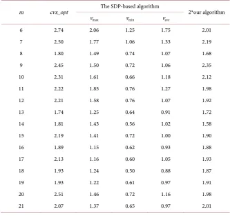
Table 1. Numerical results for n = 5, m = 6 to 30.

m cvx_opt The SDP-based algorithm 2*our algorithm

vmax vmin vave

6 2.74 2.06 1.25 1.75 2.01

7 2.50 1.77 1.06 1.33 2.19

8 1.80 1.49 0.74 1.07 1.68

9 2.45 1.50 0.72 1.06 2.35

10 2.31 1.61 0.66 1.18 2.12

11 2.22 1.85 0.76 1.27 1.98

12 2.21 1.58 0.76 1.07 1.92

13 1.74 1.25 0.64 0.91 1.72

14 1.81 1.43 0.56 1.02 1.58

15 2.19 1.41 0.72 1.00 1.90

16 1.89 1.15 0.62 0.93 1.88

17 2.13 1.16 0.60 1.05 1.93

18 1.93 1.24 0.50 0.88 1.87

19 1.93 1.22 0.61 0.97 1.91

20 2.51 1.46 0.72 1.16 1.98

(7)

DOI: 10.4236/apm.2018.84022 406 Advances in Pure Mathematics

Continued

22 2.20 1.08 0.55 0.79 1.85

23 2.13 0.99 0.55 0.81 1.95

24 1.85 0.98 0.50 0.55 1.80

25 1.92 1.28 0.70 0.98 1.91

26 1.82 0.86 0.49 0.68 1.45

27 1.88 1.05 0.54 0.73 1.76

28 1.85 1.45 0.56 0.87 1.45

29 2.39 1.25 0.44 1.02 2.30

30 1.82 1.14 0.39 0.84 1.77

The columns cvx_opt present optimal objection function values of the 20 in-stance of Pball [6]. The next two columns present the statistical results over the 10 runs of the algorithm proposed in [6] and our ACPP algorithm, respectively. The subcolumns vmax,vmin and vave give the best, the worst and the average objective function values found among 10 tests, respectively. The results show that compared with the SDP-based algorithm our algorithm is competitive in most cases.

From the table, we can see that the solution of our algorithm is very close to the exact solution of the second column, which is better than the SDP algorithm.

5. Conclusion

In this paper, we reformulate the max-min dispersion problem as a saddle point problem and then adopt an adaptive custom proximal point algorithm to obtain an approximation scheme. It can be proved that the proposed algorithm pro-duces a ε-approximation solution to the max-min dispersion problem with equal weight. Numerical results show that the proposed algorithm is efficient.

References

[1] Dasarthy, B. and White, L.J. (1980) A Maximin Location Problem. Operations Re-search, 28, 1385-1401. https://doi.org/10.1287/opre.28.6.1385

[2] Johbson, M.E., Moore, L.M. and Ylvisaker, D. (1990) Maximin Distance Designs.

Journal of Statistical Planning and Inference, 26, 131-148.

https://doi.org/10.1016/0378-3758(90)90122-B

[3] Schaback, R. (1995) Multivariate Interpolation and Approximation by Translates of A Basis Function. World Scientific, Singapore, 491-514.

[4] White, D.J. (1996) A Heuristic Approach to a Weighted Maxmin Disperation Prob-lem. IMA Journal of Management Mathematics, 7, 219-231.

https://doi.org/10.1093/imaman/7.3.219

[5] Haines, S., Loeppky, J., Tseng, P. and Wang, X. (2013) Convex Relaxations of the Weighted Maxmin Dispersion Problem. SIAM Journal on Optimization, 23, 2264-2294. https://doi.org/10.1137/120888880

(8)

DOI: 10.4236/apm.2018.84022 407 Advances in Pure Mathematics

https://doi.org/10.1137/15M1047167

[7] Ravi, S.S., Rosenkrantz, D.J. and Tayi, G.K. (1994) Heuristic and Special Case Algo-rithms for Dispersion Problems.Operations Research, 42, 299-310.

https://doi.org/10.1287/opre.42.2.299

[8] He, B. and Yuan, X. (2010) A Contraction Method with Implementable Proximal Regularization for Linearly Constrained Convex Programming. Optimization On-line, 1-14.

[9] He, B., Fu, X. and Jiang, Z. (2009) A Proximal Point Algorithm Using a Linear Proximal Term. Journal of Optimization Theory and Applications, 141, 209-239.

https://doi.org/10.1007/s10957-008-9493-0