ISSN Online: 2160-0422 ISSN Print: 2160-0414
DOI: 10.4236/acs.2018.83021 Jul. 12, 2018 318 Atmospheric and Climate Sciences
Spatio-Temporal Variability in Land Surface
Temperature and Its Relationship with
Vegetation Types over Ibadan, South-Western
Nigeria
Blessing Bolarinwa Fabeku
1*, Ifeoluwa Adebowale Balogun
2,
Suleiman Abdul-Azeez Adegboyega
2, Orimoloye Ipoola Faleyimu
11Ondo State University of Science and Technology, Akure, Nigeria 2Federal University of Technology, Akure, Nigeria
Abstract
Ibadan has experienced a rapid urbanization over the past few decades due to heavy influx of people from different parts of the country as a result of im-proved economy of the region. This development induced a great change in land use and land cover over the region which has become a major environ-mental concern recently. This study assessed Land Surface Temperature (LST) and its spatio-temporal relationship with land cover type over Ibadan. Land use/Land cover dynamics were assessed using index maps generated from Landsat Satellite data (TM, ETM+ and OLI) of Ibadan. The corrected thermal Infrared bands of the Landsat data were used to retrieve LST. The results re-vealed a notable increase in built-up areas from 5.64% of the total land cover area in 1984 to 14.05% in 2014. This change has caused increase in surface temperature of Ibadan from 3.56˚C to 8.54˚C between 1984 and 2014 respec-tively. The study recorded a continuous decrease in the vegetal part of Ibadan (from 43.28% in 1984 to 14.76 in 2014) which could be attributed to anthro-pogenic activities as the vegetated land area lost was been converted to other form of land use. The change was found to be positively correlated to the sur-face temperature intensity over the region with correlation coefficient, r value of 0.9251, 0.8256 and 0.7017 in 1984, 2000 and 2014 respectively. It is recom-mended that Policies should be considered for planting trees, new guidelines for urban landscape design and construction.
Keywords
Land Surface Temperature (LST), Land Cover Index, Normalized Differential How to cite this paper: Fabeku, B.B.,
Balo-gun, I.A., Adegboyega, S.A.-A. and Faleyi-mu, O.I. (2018) Spatio-Temporal Variabili-ty in Land Surface Temperature and Its Relationship with Vegetation Types over Ibadan, South-Western Nigeria. Atmos-pheric and Climate Sciences, 8, 318-336. https://doi.org/10.4236/acs.2018.83021
Received: April 5, 2018 Accepted: July 9, 2018 Published: July 12, 2018
Copyright © 2018 by authors and Scientific Research Publishing Inc. This work is licensed under the Creative Commons Attribution International License (CC BY 4.0).
DOI: 10.4236/acs.2018.83021 319 Atmospheric and Climate Sciences Vegetation Index (NDVI)
1. Introduction
Ibadan has experienced series of environmental change attributing to Urbaniza-tion, both in geographic extent as well as in demographic context which has transforms the landscape of the region from its natural vegetal cover types to in-creasingly impervious surface [1]. The outcome of this transformation provides a cycle of mutually reinforcing feedbacks on the climate (surface temperature increase) of the region [2] [3] [4] [5]. Continued growth in Ibadan population has resulted in drastic changes in land use/land cover pattern of the area over the past few decades [6] [7] [8]. This change enhances the incident radiation absorp-tivity, heat retention capacity and heat conductivity of the region [9], which in-turns increase the radiating surface temperature of the area [10]. The altera-tion inevitably also resulted in the redistribualtera-tion of incident radiaaltera-tion and in-duced the rural-urban surface radiance and temperature contrast.
A human induced change in the energy balance of urban environments stead-ily increases the intensity of land surface temperature (LST) which has a signifi-cant effect on observed ambient air temperature [11]. LST is one of the key pa-rameters and an important factor in the study of urban climate [12]. It varies in response to the surface energy balance, modulates the ambient air temperature, central to the energy balance of the earth surface and affects the energy ex-changes that affect the comfort of the city dwellers [13]. LST is widely used for variety of environmental studies [14] [15] [16] [17] [18] and it plays an impor-tant role in measuring surface urban heat islands, estimation of building energy consumption and evaluating heat related risks [19] [20] [21] [22]. LST had been referred to as a transient and non-uniform parameter, correlating it with a stable environmental feature like terrain and land cover becomes highly imperatives [23]. The main goal of this paper is to assess the land surface temperature and their spatio-temporal characteristic in relation to the land cover indices over the study area. The specific objectives are to examine the spatial-temporal change in the surface temperature over the study period, derive land surface temperature map reflecting the Urban Heat Island effect and investigate the relationship between the Land Surface Temperature (LST) and Land cover types over the study area.
2. Materials and Method
2.1. Study Area
DOI: 10.4236/acs.2018.83021 320 Atmospheric and Climate Sciences 2,550,593 according to 2006 census results. Until 1970, Ibadan was the largest city in sub-Saharan Africa [24] and in 1952, Ibadan was estimated to cover total land area of approximately103.8 km2[25].
Ibadan landscape consists of hard rocks and dome shaped hills gently rise from about 500 meters in the southern part, reaching a height of about 1219 m above sea level in the northern part. Its climate is equatorial, notably with dry and wet seasons with relatively high humidity. The dry season lasts from No-vember to March while the wet season starts from April and ends in October. Av-erage daily temperature ranges between 25 degrees Celsius and 35 degrees Celsius, almost throughout the year. The map of the study area is shown in Figure 1.
2.2. Data Collection
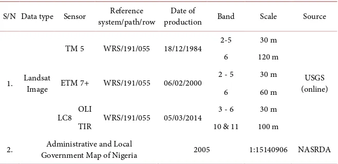
Landsat images covering the whole of Ibadan Metropolis and its eleven local government area were acquired for three different years: 1984 (Thematic Map-per), 2000 (Enhanced Thematic Mapper plus+) and 2014 (Operational Land Imager and Thermal Infra-Red Sensor) from United State Geological Survey (USGS) online archives (https://www.usgs.gov/). The local government bound-ary map and Nigerian Administrative map on the scale of 1:15,140,906 obtained from National Space Research and Development Agency, Abuja (NASRDA) was also used. The details of the data used in this study were presented in Table 1.
2.3. Data Pre-Processing
[image:3.595.218.530.533.706.2]All the Landsat datasets downloaded are cloud free and have been rectified to a common UTM (Universal Transverse Mercator) projection and WGS 84 datum. Sub-setting was done in Erdas Imagine 9.3 to limit the images to the boundary of Ibadan using the Area of Interest (AOI) created from shapefile map of the study area. Each of the sub-setted thermal bands was later resampled using the nearest neighbour algorithm in ILWIS 3.3. The thermal bands (60 meters resolution) of the downloaded Landsat Images were resampled to match the pixel size of the other bands, thus preserving 30-meter resolution of the data.
DOI: 10.4236/acs.2018.83021 321 Atmospheric and Climate Sciences Table 1. Data acquired and source.
S/N Data type Sensor system/path/row Reference production Date of Band Scale Source
1. Landsat Image
TM 5 WRS/191/055 18/12/1984 2-5 30 m
USGS (online)
6 120 m
ETM 7+ WRS/191/055 06/02/2000 2 - 5 30 m
6 60 m
LC8 OLI WRS/191/055 05/03/2014 3 - 6 30 m
TIR 10 & 11 100 m
2. Government Map of Nigeria Administrative and Local 2005 1:15140906 NASRDA
(Source: Field survey, 2016).
2.4. Data Analysis
A resampled thermal band images of Landsat 5 TM, 7 ETM+ and LC8 TIRS were used to retrieve the land surface temperature (LST) over Ibadan for the three different epochs (1984, 2000, and 2014) through the following steps:
1) Conversion of the Landsat thermal band digital numbers to at-sensor spec-tral radiance, Lλ (W∙m−2∙sr−1∙μm−1).
The spectral radiance (Lλ) for each band of was computed using the following equation [26] [27]:
(
)
LMAX LMIN DN QCALMIN LMIN
QCALMAX QCALMIN Lλ − = × − + −
(1)
for Landsat 5 TM and 7 ETM+
(
DN)
Lλ = M× +B (2)
for Landsat 8, where, DN is each pixel digital number (obtained from each thermal band), LMAX and LMIN are calibration constants, QCALMAX and QCALMIN are the highest and lowest range of values for rescaled radiance in DN. The constants values are presented on Table 2. M and B refer to the radi-ance multiplier and add values given in the header file as stipulated in Table 3.
2) Computation of the effective at-satellite brightness temperature (TB) in de-gree Kelvin.
The spectral radiance Lλ of each thermal band for the three different epochs to at-satellite brightness temperature TB conversion under the assumption of uni-form emissivity was done using the following uni-formula [26]:
2 1 ln 1 B K T K Lλ = + (3)
DOI: 10.4236/acs.2018.83021 322 Atmospheric and Climate Sciences Table 2. ETM+ and TM thermal band calibration constants.
Satellite/sensor Band Lmin Lmax Qcalmin Qcalmax (w/m2K/sr/μm) 1
K2
(degree Kelvin) Landsat 5 TM 6 1.238 15.600 0.0 255.0 607.76 1260.56
Landsat 7 ETM+ 61 0.000 17.040 1.0 255.0 666.09 1282.71 62 3.200 12.650 1.0 255.0
(Source: [26]).
Table 3. The Metadata of Landsat 8-TIR.
Landsat 8 Band 10 Band 11
Radiance Multiplier (M) 0.0003342 0.0003342
Radiance Add (A) 0.1 0.1
K1 774.89 480.89
K2 1321.08 1201.14
Source: [28] [29]; where K2 and K1 are pre-launch calibration constants of Landsat Sensor Used.
radiance in W/m2/sr/μm, K
2 and K1 are pre-launch calibration constants, the value for this constant are presented in Table 2 and Table 3.
3) Estimation of land surface emissivity.
The temperature values obtained above using Equation (3) are referenced to a blackbody. There is need for spectral emissivity (ε) corrections in respect to the nature of land cover type. The emissivity of a heterogeneous surface was com-puted using Equations [30]:
(
1)
vλ fv sλ fv Cλ
ε ε
= × +ε
× − + (4)2 s
v s
NDVI NDVI
NDVI NVDI
v
f = −−
(5)
NIR RED NDVI
NIR RED
− =
+ (6)
(
1 s)
v(
1 v)
Cλ = −
ε
λ ×ε
λ× × −F′ f (7)where; εs and εv are the emissivity (ε) of soil pixels and full vegetation pixels with the mean value of 0.97 and 0.99 respectively [30], fv is the proportion of vegetation in each pixel which was estimated using Equation (5) [30], NDVI is the Normalized Differential Index and it was calculated using algorithm (Equa-tion (6)) developed by [31]. NIR and R are the reflectance in the near-infrared (band 4) and red (band 3) portion of the electromagnetic spectrum respectively. NDVIs and NDVIv is Normalized Difference Vegetation Index Thresholds value for soil pixels (NDVIs=0.2), and pixels of full vegetation (NDVIv=0.5)
[image:5.595.309.536.455.566.2]DOI: 10.4236/acs.2018.83021 323 Atmospheric and Climate Sciences value of 0.55 [32].
4) Calculation of final temperature at the surface or on the ground (LST) in degree Celsius.
Finally, the land surface temperature (Stemp) in degrees Celsius was computed as follows [34]:
(
)
273.151 B ln
temp
B T S
T
λ
ρ
ε
= −
+ × × (8)
where; TB is effective at-satellite temperature in degree Kelvin as computed in Equation (3), λ = wavelength of emitted radiance (for which the peak response and the average of the limiting wavelengths (λ = 11.45 μm) [35] was used,
h c
ρ= × σ (1.438 × 10⁻² m∙K), σ = Boltzmann constant (1.38 × 10⁻²³ J/K), h = Planck’s constant (6.626 × 10⁻³⁴ J∙s), and c = velocity of light (2.998 × 10⁸ m/s). ε is the emissivity of a mixed pixels as estimated using Equation (4).
For each of the studied years (that is, 1984, 2000 and 2014), an emissivi-ty-corrected land surface temperature (LST) maps in degree Celsius were re-trieved from Resampled-Landsat thermal bandimages (Figure 2(a)). The LST maps produced shows the spatio-temporal variability and distribution of the land surface temperature over the study.
2.5. Land Surface Temperature/Land Cover Type Relationship
(Correlation Analysis)
− LST versus Normalized Differential Vegetation Index (NDVI). − LST versus Built-Up Index (BUI).
To investigate the Land Surface Temperature-Land Cover type relationship (both sample maps were resampled to a common spatial resolution, 30 m) and how it varies over the study area for the period considered, the land cover types were classified intotwo distinct parts; the built-up area and the vegetal part. In respect of this classification, two land cover indices (LC); Built-Up Area Index (BUI) and Normalised Differential Vegetation Index (NDVI) maps were gener-ated using ILWIS 3.5 from Landsat imagery (Figure 3(a) and Figure 3(b)). Both LST and LC index maps (that is, NDVI and BUI) were gridded at a regular in-terval (5 km), 46 squares, were randomly selected. The mean value of the data extrapolated from each of this square. LST values were plotted against each the corresponding NDVI, BUI values using Microsoft Excel and a regression graph was obtained for each of the years (1984, 2000 and 2014) considered in this study.
The mean values of the extracted LST data were compared to that of NDVI and BUI respectively in each repression relation through correlation coefficients, r [36] and coefficient of determinant, r2 [37].
(
)(
)
(
) (
)
{
1 ,NDVI/BUI NDVI/BUI2 ,LST LST 2}
,NDVI/BUI NDVI/BUI ,LST LST
1 n i i i n i i i
X X Y
r Y Y X X Y = = − − = − −
∑
DOI: 10.4236/acs.2018.83021 325 Atmospheric and Climate Sciences (b)
DOI: 10.4236/acs.2018.83021 327 Atmospheric and Climate Sciences (b)
DOI: 10.4236/acs.2018.83021 328 Atmospheric and Climate Sciences
(
)
(
)
2 NDVI/BUI LST 2 1 2 NDVI/BUI NDVI/BUI 1 1 n i n i X Y r X X = = − = − −∑
∑
(10)where, Xi,NDVI/BUI and XNDVI/BUI are NDVI/BUI values (independent variable)
extracted from each pixel within a particular square and the mean value of same variable for each square respectively. Yi,LST and YLST are LST values (dependent
variable) extracted from each corresponding pixel within a particular square and the mean value of same variable for each square respectively.
2.6. Generation of Land Cover Type Index Map Using NDVI and
BUI Algorithm
The most commonly used index for monitoring vegetation distribution is Nor-malised Differential Vegetation Index (NDVI) [38] as computed using Equation (6). Another applied indicator of development and vegetation distribution, Built-Up Index (BUI) was computed using the following equation [39]:
BUI NDBI NDVI= − (11)
SWIR NIR NDBI
SWIR NIR
− =
+ (12)
where, NDBI is Normalised Differential Built-Up Index (NDBI), useful for monitoring the distribution of urban areas [40]. SWIR and NIR is the reflectance in the short wave infrared band (band 5 for TM and ETM+, band 6 for LC8 OLI) and reflectance in the near-infrared band of electromagnetic spectrum respec-tively. The Built-Up Index map distinguished between non-urban and urban ar-eas based on their index values. Urban arar-eas are associated with high BUI values while non-urban areas have low BUI values.
Script was writing for all the formulas used in the methodology and run per-fectly using Script Editor in ILWIS 3.5 and the selected outputs for this study were LST maps, NDVI map and BUI map for each of the years; 1984, 2000 and 2014 as presented under results.
3. Results and Discussion
3.1. Spatio-Temporal Variability and Distribution of the Land
Surface Temperature (LST)
DOI: 10.4236/acs.2018.83021 329 Atmospheric and Climate Sciences compared to its previous status in 1984 which was as a result of transformation of the area which used to be a forest into arable land. The situation seems to be getting worse as it was observed from Figure 2(a-iii) that more area is been af-flicted by high surface temperature and not only that, the temperature value is also getting intense.
Comparison study demonstrated between the Land use/Land cover Index map (Built-Up Index map and Normalised vegetation differential index map) and Land Surface Temperature map revealed that the vegetal part of the study area are directly linked to area of lower temperature values while the area associated with high temperature values are built-up area, areas of human activities like construction, cultivation, mining, logging, burning etc. and impervious surfaces. This result was in conformity with other studies [41] [42] which has proven that surface temperature will always be lesser over the vegetation compare to bare or exposed soil, because the canopy intercepts the incoming solar radiation (short wave), reflect little and absorbs substantial amount which is converted to chemical energy that aids photosynthesis with the help of chlorophyll and loses it excess energy to the process of evapotranspiration [43]. So, less incoming ra-diation actually get to the surface and little will be emitted back to the atmos-phere. But bare surface has nothing to intercept the incoming shortwave radia-tion, so it absorb more incoming energy and emits more to the surrounding in form of long wave thereby increase the temperature value of the near surface air.
Also most of the building materials used in Ibadan not only within the city but the suburbs has varying capacity of physical surface properties (albedo, thermal capacity, and heat conductivity) that acts as a major contributing factor to the environment temperature increase. Commonly used in Ibadan for roofing is the galvanized iron sheet, which used to be a shining surface material that reflect more of the incoming radiation, transforms over the years due to rusting and this had in turn change their physical properties and caused them to absorb more of radiation than reflecting. This scenario will cause more emission of long wave and thereby contribute more to the surface temperature.
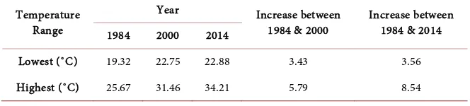
[image:12.595.208.540.653.728.2]The spatio-temporal land surface temperature difference as portrayed by Fig-ure 2 over the three epochs (1984, 2000 and 2014) considered in this study were summarized in Table 4. The table depicts that between 1984 and 2000, the minimum temperature has increased by 3.43˚C and the maximum temperature by 5.79˚C while over the past three decades, and rural temperature has further increased by 3.56˚C and that of urban area by 8.54˚C.
Table 4. Land surface temperature value range over the years.
Temperature Range
Year Increase between
1984 & 2000 Increase between 1984 & 2014 1984 2000 2014
Lowest (˚C) 19.32 22.75 22.88 3.43 3.56
DOI: 10.4236/acs.2018.83021 330 Atmospheric and Climate Sciences The findings that the urban area, the arable land and other part where there is development are associated with high land surface temperature while the rural part with more of vegetation and water bodies corresponds to low temperature was in line with Seema and Sharma (2014) report [29], which reveals that highest Land Surface Temperature (LST) corresponds to bare soil area, built-up areas and agricultural fallow land. Water bodies record lowest LST values followed by vegetation classes. Related result was also presented by Weng et al., (2004) [9], where it was noted that commercial and industrial land exhibited the highest temperature, followed by residential land. The lowest temperature was observed in the forest area followed by water bodies.
3.2. Land Surface Temperature/Land Cover Type Relationship
Correlation analysis was demonstrated on Built-Up Area-Land Surface Tem-perature (BUI-LST) map and Normalized Differential Vegetation Index-Land Surface Temperature (NDVI-LST) map respectively, and Figures 4(a)-(f) were obtained. The summary of this analysis is presented in Table 5.It could be noted from Table 5 that LST and BUI show a strong positive cor-relation in 1984 as the rvalue of 0.9251 was obtained. Also in the year 2000, r value of 0.8256 was observed from LST-BUI plot which indicate strong positive correlation. The year 2014 was no exception as the correlation coefficient, r value between LST and BUI was 0.7017 meaning they are strongly positively corre-lated. The result show that there exist a positive correlation between the land surface temperature and the built-up area index values, which means there is a linear relationship between them and either of the two (LST value and BUI value) can be used to predict the intensity of the other. This also meant the ad-vancement in the built-up area will definitely increase the intensity of the land surface temperature in Ibadan locality.
[image:13.595.199.540.611.734.2]The same Table 5 revealed the correlation coefficient, r values exist between LST and NDVI maps for the three different years to be −0.8840, −0.8056 and −0.6361 for the year 1984, 2000 and 2014 respectively. This result shows that there is a strong correlation between LST and NDVI but they are inversely re-lated. This result on the other hand shows that land surface temperature and
Table 5. Coefficient of determinant and coefficient of correlation of LST versus BUI and NDVI index; Note: +value means linear relationship while –value means inverse rela-tionship.
Year
LST Versus BUI LST Versus NDVI
Coefficient of determinant
r2
Coefficient of correlation
r
Coefficient of determinant
r2
Coefficient of correlation
r
1984 0.8558 0.9251 −0.7814 −0.8840
2000 0.6816 0.8256 −0.6490 −0.8056
DOI: 10.4236/acs.2018.83021 331 Atmospheric and Climate Sciences (a)
(b)
DOI: 10.4236/acs.2018.83021 332 Atmospheric and Climate Sciences (d)
(e)
[image:15.595.227.518.71.643.2](f)
DOI: 10.4236/acs.2018.83021 333 Atmospheric and Climate Sciences normalised differential vegetation index are inversely related, which means the improvement in vegetation of any geographical location will definitely reduce the intensity of the land surface temperature over the region. This could be used as measure to ameliorate the effect of Urban Heat Island. It is also important to note that there exist an inverse relationship observed between BUI and NDVI from Figure 3(a) and Figure 3(b). In Nigeria, environmental development en-courages cutting down of trees which have an adverse effect on the vegetation.
The result that LST maintain an inverse relationship with NDVI and linear relationship with BUI was similar to the findings of Seema and Kavita (2014)
[29], which reported that the statistics underlines significant negative relation-ship between LST and abundance of vegetation cover. The correlation between the LST and NVDI images was reported to be −0.562 in 2000 and −0.522 in 2011. Weng et al., (2014) also noted a similar result that both vegetation indica-tors considered in their study show the strong, negative correlation with LST and the highest negative correlation was found in cropland and forest.
4. Conclusion
This study has found significant proof of continuous increase in land surface temperature and effect of Urban Heat Island over Ibadan. Urban development had an adverse effect on the vegetation by contributing greatly to its depletion, in which the process in-turns intensified the warming of the immediate sur-roundings. The manner in which Ibadan develops over the coming decades will play a critical role in determining the characteristics of its environmental tem-perature under climate change. It is expected that as the city expands further, the magnitude of the land surface temperature would become stronger affecting the living conditions of the urban population. There exists an inverse relationship between the LST and vegetative area cover while LST Index and Built-Up Area Index maintain a linear positive relationship. This relationship between urban temperature and land cover types helps to find out the best solutions for urban environment quality improvement and the planning strategies for heat island reduction. These strategies are essential for the future of urban development as it may become necessary to apply these solutions to reduce the harmful impacts of increasing temperatures and the urban heat island.
References
[1] Kafi, K.M., Shafri, H.Z.M. and Shariff, A.B.M. (2014) An Analysis of LULC Change Detection Using Remotely Sensed Data; A Case Study of Bauchi City. IOP Confer-ence Series: Earth and Environmental Science, 20, 12-56.
[2] Landsberg, H.E. (1981) The Urban Climate. Academic Press, New York.
DOI: 10.4236/acs.2018.83021 334 Atmospheric and Climate Sciences Press, Cambridge, 499-587.
[4] Bonan, G.B. (2008) Forests and Climate Change: Forcings, Feedbacks and the Cli-mate Benefits of Forests. Science, 320, 1444-1449.
https://doi.org/10.1126/science.1155121
[5] McCarthy, M.P., Best, M.J. and Betts, R.A. (2010) Climate Change in Cities Due to Global Warming and Urban Effects. Geophysical Research Letters, 37, L09705.
https://doi.org/10.1029/2010GL042845
[6] Weng, Y.C. (2007) Spatiotemporal Changes of Landscape Pattern in Response to Urbanization. Landscape and Urban Planning, 81, 341-353.
https://doi.org/10.1016/j.landurbplan.2007.01.009
[7] Turkoglu, N. (2010) Analysis of Urban Effects on Soil Temperature in Ankara. En-vironmental Monitoring and Assessment, 169, 439-450.
https://doi.org/10.1007/s10661-009-1187-z
[8] Mosammam, H.M., Nia, J.T., Khani, H., Teymouri, A. and Kazemi, M. (2016) Monitoring Land Use Change and Measuring Urban Sprawl Based on Its Spatial Forms: The Case of Qom City. The Egyptian Journal of Remote Sensing and Space Science,20, 103-116. https://doi.org/10.1016/j.ejrs.2016.08.002
[9] Weng, Q., Lub, D. and Schubring, J. (2004) Estimation of Land Surface Tempera-ture-Vegetation Abundance Relationship for Urban Heat Island Studies. Remote Sensing of Environment, 89, 467-483. https://doi.org/10.1016/j.rse.2003.11.005
[10] Khandelwal, S., Goyal, R. and Mathew, A. (2017) Assessment of Land Surface Tem-perature Variation Due to Change in Elevation of Area Surrounding Jaipur, India. The Egyptian Journal of Remote Sensing and Space Science,21, 87-94.
https://doi.org/10.1016/j.ejrs.2017.01.005
[11] Oluseyi, O.F. (2006) Urban Land Use Change Analysis of a Traditional City from Remote Sensing Data: The Case of Ibadan Metropolitan Area, Nigeria. Humanities and Social Sciences Journal, 1, 42-64.
[12] Pu, R., Gong, P., Michishita, R. and Sasagawa, T. (2006) Assessment of Multi-Resolution and Multi-Sensor Data for Urban Surface Temperature Retrieval. Remote Sensing of Environment, 104, 211-225. https://doi.org/10.1016/j.rse.2005.09.022
[13] Voogt, J.A. and Oke, T.R. (2003) Thermal Remote Sensing of Urban Climates. Re-mote Sensing of Environment, 86, 370-384.
https://doi.org/10.1016/S0034-4257(03)00079-8
[14] Running, S.W., Justice, C., Salomonson, V., Hall, D., Braker, J., Kaufman, Y., Strahler, A., Huete, A., Muller, J.P., Vanderbilt, V., Wan, Z. and Teillet, P. (1994) Terrestrial Remote Sensing Science and Algorithms Planned for EOS/MODIS. In-ternational Journal of Remote Sensing, 15, 3587-3620.
https://doi.org/10.1080/01431169408954346
[15] Vining, R.C. and Blad, B.L. (1992) Estimation of Sensible Heat Flux from Remotely Sensed Canopy Temperatures. Journal of Geophysical Research, 97, 18951-18954.
https://doi.org/10.1029/92JD01626
[16] Diak, G.R. and Whipple, M.S. (1995) Note on Estimating Surface Sensible Heat Fluxes Using S, L Measured from a Geostationary Satellite during FIFE 1989. Jour-nal of Geophysical Research, 100, 25453-25461. https://doi.org/10.1029/95JD00729
[17] Crago, R., Sugita, M. and Brutsaert, W. (1995) Satellite-Derived Surface Tempera-tures with Boundary Layer TemperaTempera-tures and Geostrophic Winds to Estimate Sur-face Energy Fluxes. Journal of Geophysical Research, 100, 25447-25451.
DOI: 10.4236/acs.2018.83021 335 Atmospheric and Climate Sciences [18] Kimura, F. and Shimiru, A.P. (1994) Estimation of Sensible and Latent Heat Fluxes from Soil Surface Temperatures Using a Linear Air Land Heat Transfer Model. Journal of Applied Meteorology, 33, 477-489.
https://doi.org/10.1175/1520-0450(1994)033<0477:EOSALH>2.0.CO;2
[19] Weng, Q. and Fu, P. (2014) Modelling Annual Parameters of Land Surface Tem-perature Variations and Evaluating the Impact of Cloud Cover Using Time Series of Landsat TIR Data. Remote Sensing of Environment, 140, 267-278.
https://doi.org/10.1016/j.rse.2013.09.002
[20] Hu, L. and Brunsell, N.A. (2013) The Impact of Temporal Aggregation of Land Surface Temperature Data for Surface Urban Heat Island (SUHI) Monitoring. Re-mote Sensing of Environment, 134, 162-174.
https://doi.org/10.1016/j.rse.2013.02.022
[21] Deng, C. and Wu, C. (2013) Examining the Impacts of Urban Biophysical Compo-sitions on Surface Urban Heat Island: A Spectral Unmixing and Thermal Mixing Approach. Remote Sensing of Environment, 131, 262-274.
https://doi.org/10.1016/j.rse.2012.12.020
[22] Mathew, A., Sreekumar, S., Khandelwal, S., Kaul, N. and Kumar, R. (2016) Predic-tion of Surface Temperatures for the Assessment of Urban Heat Island Effect over Ahmedabad City Using Linear Time Series Model. Energy and Buildings, 128, 605-616. https://doi.org/10.1016/j.enbuild.2016.07.004
[23] Fan, X.M., Liu, H.G., Liu, G.H. and Li, S.B. (2014). Reconstruction of MODIS Land-Surface Temperature in a Flat Terrain and Fragmented Landscape. Interna-tional Journal of Remote Sensing, 35, 7857-7877.
https://doi.org/10.1080/01431161.2014.978036
[24] Lloyd, P.C., Mabogunje, A.L. and Awe, B. (1967) The City of Ibadan. Cambridge University Press, Cambridge.
[25] Areola, O. (1994) The Spatial Growth of Ibadan City and Its Impact on the Rural Hinterland. In: Filani, M.O., Akintola, F.O. and Ikporukpo, C.O., Eds., Ibadan Re-gion, Rex Charles Publication, Ibadan, 72-84.
[26] Landsat Project Science Office (2002) Landsat 7 Science Data User’s Handbook. Goddard Space Flight Center, NASA, Washington DC.
https://landsat.usgs.gov/landsat-7-data-users-handbook
[27] Chander, G. and Markham, B. (2003) Revised Landsat-5 TM Radiometric Calibra-tion Procedures and Post CalibraCalibra-tion Dynamic Ranges. IEEE Transactions on Geo-science and Remote Sensing, 41, 2674-2677.
https://doi.org/10.1109/TGRS.2003.818464
[28] USGS (2013) Using the USGS Landsat 8 Product.
https://landsat.usgs.gov/using-usgs-landsat-8-product
[29] Seema, J. and Kavita, S. (2014) Spatio-Temporal Assessment of Land Use/Land Cover Dynamics and Urban Heat Island of Jaipur City Using Satellite Data. The In-ternational Archives of the Photogrammetry, Remote Sensing and Spatial Informa-tion Sciences, 40, 767-772.
[30] Sobrino, J.A., Jimenez-munoz, J.C., El-kharraz, J., Gomez, M., Romaguera, M. and Soria, G. (2004) Single-Channel and Two-Channel Methods for Land Surface Tem-perature Retrieval from DAIS Data and Its Application to the Barrax Site. Interna-tional Journal of Remote Sensing, 25, 215-230.
https://doi.org/10.1080/0143116031000115210
Sympo-DOI: 10.4236/acs.2018.83021 336 Atmospheric and Climate Sciences sium, Washington DC, date, 309-317.
[32] Sobrino, J.A., Caselles, V. and Becker, F. (1990) Significance of the Remotely Sensed Thermal Infrared Measurements Obtained over a Citrus Orchard. ISPRS Photo-grammetric Engineering and Remote Sensing, 44, 343-354.
https://doi.org/10.1016/0924-2716(90)90077-O
[33] Sobrino, J.A., Jiménez-Muñoz, J.C., Sòria, G., Romaguera, M., Guanter, L. and Mo-reno, J. (2008) Land Surface Emissivity Retrieval from Different VNIR and TIR Sensors. IEEE Transactions on Geoscience and Remote Sensing, 46, 316-327. [34] Artis, D.A. and Carnahan, W.H. (1982) Survey of Emissivity Variability in
Ther-mography of Urban Areas. Remote Sensing of Environment, 12, 313-329.
https://doi.org/10.1016/0034-4257(82)90043-8
[35] Markham, B.L. and Barker, J.L. (1985) Spectral Characterization of the Landsat Thematic Mapper Sensors. International Journal of Remote Sensing, 6, 697-716.
https://doi.org/10.1080/01431168508948492
[36] Almorox, J., Bocco, M. and Willington, E. (2013) Estimation of Daily Global Solar Radiation from Measured Temperatures at Cañada de Luque, Córdoba, Argentina. Renewable Energy, 60, 382-387. https://doi.org/10.1016/j.renene.2013.05.033
[37] Ouali, K. and Alkama, R. (2014) A New Model of Global Solar Radiation Based on Meteorological Data in Bejaia City (Algeria). Energy Procedia, 50, 670-676.
https://doi.org/10.1016/j.egypro.2014.06.082
[38] Jensen, J.R. (2000) Remote Sensing of the Environment: An Earth Resource Per-spective. Pearson Education, Inc., Delhi, 361-365.
[39] Zhang, Y., Odeh, I.O.A. and Han, C. (2009) Bi-Temporal Characterization of Land Surface Temperature in Relation to Impervious Surface Area, NDVI and NDBI Us-ing a Subpixel Image Analysis. International Journal of Applied Earth Observation and Geoinformation, 11, 256-264. https://doi.org/10.1016/j.jag.2009.03.001
[40] Griffiths, T.L., Chater, N., Kemp, C., Perfors, A. and Tenenbaum, B. (2010) Prob-abilistic Models of Cognition: Exploring Representations and Inductive Biases. Trends in Cognitive Sciences, 14, 357-364. https://doi.org/10.1016/j.tics.2010.05.004
[41] Gallo, K.P. and Tarpley, J.D. (1996) The Comparison of Vegetation Index and Sur-face Temperature Composites of Urban Heat-Island Analysis. International Journal of Remote Sensing, 17, 3071-3076. https://doi.org/10.1080/01431169608949128
[42] Weng, Q. (2001) A Remote Sensing-GIS Evaluation of Urban Expansion and Its Impact on Surface Temperature in the Zhujiang Delta, China. International Journal of Remote Sensing, 22, 1999-2014.