ISSN Online: 2160-5920 ISSN Print: 2160-5912
Classifying Hand Written Digits with Deep
Learning
Ruzhang Yang
Shanghai Foreign Language School, Shanghai, China
Abstract
Recognizing digits from natural images is an important computer vision task that has many real-world applications in check reading, street number recog-nition, transcription of text in images, etc. Traditional machine learning ap-proaches to this problem rely on hand crafted feature. However, such features are difficult to design and do not generalize to novel situations. Recently, deep learning has achieved extraordinary performance in many machine learning tasks by automatically learning good features. In this paper, we investigate using deep learning for hand written digit recognition. We show that with a simple network, we achieve 99.3% accuracy on the MNIST dataset. In addi-tion, we use the deep network to detect images with multiple digits. We show that deep networks are not only able to classify digits, but they are also able to localize them.
Keywords
Digit Classification, Deep Network, Gradient Descent
1. Introduction
Text recognition from images is an important task that has multiple real-world applications such as text localization [1] [2], transcription of text into digital format [3] [4], car plate reading [5] [6] [7] [8], automatic check reading [9], classifying text from unlabeled/partially labeled documents [10], recognizing road signs and house number [11][12], etc. Traditionally hand designed features are used to for image classification [13][14][15][16][17]. However, these tech-niques require a huge amount of engineering effort, and often do not generalize to novel situations.
Recent techniques in deep learning have allowed efficient automatic learning of features that are superior to hand designed features. As a result, we are able to
How to cite this paper: Yang, R.Z. (2018) Classifying Hand Written Digits with Deep Learning. Intelligent Information Man-agement, 10, 69-78.
https://doi.org/10.4236/iim.2018.102005
Received: March 2, 2018 Accepted: March 25, 2018 Published: March 28, 2018
Copyright © 2018 by author and Scientific Research Publishing Inc. This work is licensed under the Creative Commons Attribution International License (CC BY 4.0).
http://creativecommons.org/licenses/by/4.0/ Open Access
train classifier that is significantly more accurate compared to previous methods. In this paper, we investigate using deep learning to classify handwritten digits, and show that with a simple deep network, we can classify digits with near-perfect accuracy.
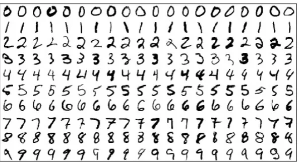
We test our methods on the MNIST dataset [18]. This dataset consists of 50,000 training digit images and 10,000 testing images and is an important benchmark for deep learning methods. Samples images from the dataset are shown in Figure 1. On this dataset, we achieve an accuracy of 99.3% on the test set.
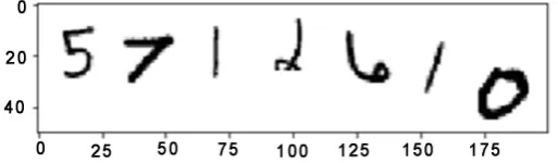
We also investigate classifying multiple digits, where more than one digit is present in an image. An example of this task is shown in Figure 2. We design a novel method of applying classifier of a single digit to an image with multiple di-gits. Though the number of digits and their location is unknown a-priori, our method is able to accurately localize and classify all the digits in the image.
2. Digit Classification with Deep Networks
2.1. Supervised Learning
A supervised learning task consists of two components, the input x and label y. For example, the input can be images of handwritten digits, or image of natural objects, and the label is the corresponding digit class or object class. The goal is to learn the correct mapping f from input x to label y. To accomplish this a learner is provided with examples of the correct mapping
(
x yi, i)
,i=1,,N where xi is an example input and yi is the corresponding label provided by hu-man annotators. Ideally after learning, f should map each input in the dataset(
x yi, i)
,i=1,,N to the correct label, i.e.f(xi) = yi. The hope is that the learner can learn the correct mapping between x and y based on these examples, so that on unseen data, the learner f can also correctly classify.Usually f is selected from a class of functions indexed by a parameter θ. For example, the class of functions can be quadratic functions
( )
2 [image:2.595.226.523.536.697.2]f x =ax +bx+c
Figure 1. Samples from the MNIST dataset.
Figure 2. Classifying multiple digits.
in this example,
θ
=(
a b c, ,)
are the parameters. We will denote the function selected by a parameter choice as fθ.To encourage the learner to select a fθ that maps each xi to the correctyi we define a loss function such as
( )
(
)
21 N
i i
i
f x y
θ θ
=
=
∑
−
In general any loss function that takes a smaller value when f(xi) is closer to yi can be used. For classification tasks we use a special class of functions fθ that
outputs a probability distribution. That is for each xi,
( )
ji
fθ x is the
probabil-ity the input belongs to the j-th class. Then we can use the cross-entropy loss
(
)
( )
1
log K
j
i i
j
Lθ I y j fθ x
=
=
∑
=where K is the number of classes, and I y
(
j = f)
=1 if yi = j and equals to 0 otherwise.To train the model, we use gradient descent on the loss function Lθ. This is described by the following process:
1) We start from a random parameter θ that can be arbitrarily chosen. 2) We compute the gradient of the loss function ∇θLθ. Computation of this
gradient is discussed in the next section.
3) We update the parameters by θ: = θ − α∇θLθ. This changes θ in the direc-tion that minimizes the loss Lθ. α is the learning rate that controls the step size. The larger the step size, the faster θ changes. However, step size that is too large may lead to instability or even divergence. Therefore, the learning rate α is an important hyperparameter that is selected based on the specific problem.
4) We repeat from Step 2 until θ stops changing.
The above algorithm reduces Lθduring each iteration. The hope is that when
Lθis minimized, fθ(xi) will be close to yi, that is, the function fθwe selected can correctly predict the label yigiven xion the training set.
However, even if fθcorrectly predicts every example we provided, this does not mean that fθwill classify correctly on new data. For example, fθ may have only memorized the training dataset. Therefore we need additional examples (xj,yj), j=1,,M that the learner has not seen during training. The learner should only be able to classify these new examples correctly if it has learned the
correct mapping between x and y. We can compute the testing accuracy by di-viding the number of examples fθcorrectly classifies by the total number of ex-amples. This is the final measurement of performance that we use to evaluate our learner.
2.2. Deep Networks
In the previous section we left an open question: which class of functions
{ }
fθto select from during training. This section introduces an important function class of deep networks [19][20][21].
The key idea of deep learning is to compose very simple functions 1 2
1 2
, ,
d
d
gθ gθ gθ
into a very complex function
( )
(
1(
2(
1( )
)
)
)
1 2 1
d d
d d
x g g g x
fθ = θ θ−− gθ θ . Each function
i
i
gθ is a simple function with parameters θi. Then the parameters of f is simply
the combined parameters of all the layers
θ
=(
θ
1,,θ
d)
. Common functions used in deep learning include1) Matrix multiplication g(x) = Ax + b where the parameters are matrix A and vector b.
2) Rectified Linearity (ReLU) [22]
( )
00 x x g x o x > = <
This function does not contain a parameter.
3) Softmax function: the softmax function “squashes” a n-dimensional vector of arbitrary real values to a n-dimensional vector of real values in the range [0, 1] that add up to 1. The function applied to an n-dimensional input vector z is given by
( )
1 e Sigmoid e j k z n Z j k z = =∑
Note that sigmoid naturally produces a distribution because the output sum to 1
( )
Sigmoid j 1
j
z =
∑
4) Convolution [23][24][25][26]: the convolution function takes as input an array z of size M × N × K and output an array o of size M × N × C. The first two dimensions can be interpreted as width and height, while the third is the number of “channels”. This function takes the input z, and applies a 2D-convolution op-eration defined as
, , , , , ,
0 0
, 1 , , , ,
S S
c
x y c i j k x i y j k
i i
o w z + + x y c M N C
= =
=
∑∑
∗ ∀ ≤ ≤where S is called the size of the filter map, and each c
w is an array of size S × S
× K. All the c
w combined
{
wc,c=1,,C}
is the set of parameters of theconvolution function.
5) Pooling: Pooling is a process which reduces a M × N × K array into a smaller array, e.g. of size M 2×N 2×C. Usually we keep the number of
“channels” unchanged. For example, in the digit classification task, it can reduce the scale of a clearer picture into a more ambiguous one, making it easier to process in the later steps.
We shall denote the output of
(
( )
1)
1 i
i
gθ gθ as hi. Then
( )
d(
1)
dd
fθ x =gθ h− ,
(
)
1 1
1 d 2
d
d d
h gθ− h
−
− = − etc. Finally, we have 1
( )
1 1h =gθ x . Intuitively the network
must map raw input images into highly abstract and meaningful labels, which is a highly complex mapping. The network accomplishes through a sequence of simple mappings composed together. Each function i
i
gθ can be viewed as one
“layer” of a network. This function i
gθ processes the output of the previous
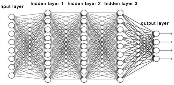
functions hi−1 into higher level representations hi. The network therefore can be viewed as processing the input through a sequence of “layers” whose output be-come increasingly more high level and abstract, until we finally reach the output layer, which corresponds to the labels. This intuition is illustrated in Figure 3.
2.3. Computing Gradients
Now that we have defined our model class, to implement the algorithm in Sec-tion 2.1, we must be able to compute the gradient ∇θLθ. This is accomplished with the back-propagation algorithm [19][20][21].
The back-propagation algorithm sequentially computes
1 1
, ,, .
yLθ hd−Lθ hLθ
∇ ∇ ∇ Intuitively, this tells us how each hidden layer must
change to minimize loss Lθ. When all the i
i
gθ are simple functions, we can
compute ∇hi−1Lθfrom ∇hiLθanalytically, and this can be computed automatically by software such as Tensorflow [27]. Given gradient ∇hiLθover each layer hi, we can correspondingly compute the gradient ∇θiLθover parameters θi analytically. This can also be automatically computed by Tensorflow.
Intuitively the computation flows “backward” through the next (hence the name back-propagation). We compute gradient in the following sequence
1 1 1 1
, , , , , ,
yLθ θdLθ hd−Lθ θd−Lθ hLθ θ Lθ
∇ ∇ ∇ ∇ ∇ ∇
2.4. Detecting and Localizing Multiple Digits
In many real-world problems, such as car plate detection [5][6][7][8] or house number recognition [11] there are multiple digits in the same image, and their location is unknown to us. Therefore, not only do we want to classify existing digits, we would also like to locate where the digits are, and how many there are. We show that based on the deep classifier we trained before we can design an algorithm to accomplish this. What we need is that given an image patch we must identify both whether there is a digit in the image patch, and what digit it is, if there is one. If we can accomplish this, then we may simply apply this me-thod to each patch of our input image, and we will be able to localize and classify all the digits in the image.
Previously we trained a classifier fθ
( )
x that takes as input an image, andoutputs a probability distribution over all possible digits. We observe that when the input is an image that do not contain any digit, the output is a distribution
Figure 3. Illustration of a deep network.
with high entropy, that is, the network is not highly confident that any digit has been observed. On the other hand, when presented with an image that contains a digit, the output is a distribution with low entropy, and the network generally outputs the correct digit with very high confidence.
We can then take advantage of this property. We measure the difference be-tween the highest probability score and the second highest probability score. If the image contains a digit, the top prediction should have high probability score compared to the second highest. If the image does not contain a digit, all the possible predictions should be assigned similar probability and there should not be a significant difference. We show that this approach works very well in prac-tice and we are able to accurately discover digits in an image in the experiments.
3. Experiment
3.1. Experiment Setting
We use 50,000 digit figures from the MNSIT training dataset to accomplish our training. Each example is a 28 by 28 single-color image. Our network architec-ture is as follows
1) A convolution layer with filter map of size 5 that takes as input the 28 × 28 × 1 image and outputs a feature map of shape 28 × 28 × 32
2) A pooling layer that reduces the size from 28 × 28 × 32 to 14 × 14 × 32 3) A ReLU layer
4) A convolution layer with filter map of size 5 and outputs a feature map of shape 14 × 14 × 64
5) A pooling layer that reduces the size from 14 × 14 × 64 to 7 × 7 × 64 6) A matrix multiplication layer that maps a vector of size 7 × 7 × 64 to 1024 7) A ReLU layer
8) A matrix multiplication layer that maps a vector of size 1024 to 10 9) A softmax layer
We train our network with gradient descent with a learning rate of 4 1e− for
20,000 iterations. We also use a new adaptive gradient descent algorithm known as Adam [28] which has been shown to perform better on a variety of tasks. Be-cause shifting a digit does not change its class, during training we also randomly shift the digit by up to 6 pixels in each direction to augment the dataset. This makes the network more robust to shifting of the digit and improves testing ac-curacy.
For multi-digit classification, we first extract all 28 by 28 image patches with a stride of 2. Then we run our classification network on all the patches, we take the most confident digit prediction in a region as our digit class prediction.
3.2. Results
3.2.1. Single Digit Classification
After training our network, we use another 10,000 test data to test the accuracy of our network. We achieved a testing accuracy of 0.993, which indicates that the network only makes a mistake in 7 out of every 1000 digits. We show the train-ing curve in Figure 4. It can be observed that accuracy improves very quickly in the first 5000 iterations, then improves gradually until we reach approximately 99% accuracy on both the training set and testing set. No overfitting is observed.
3.2.2. Multiple Digit Classification
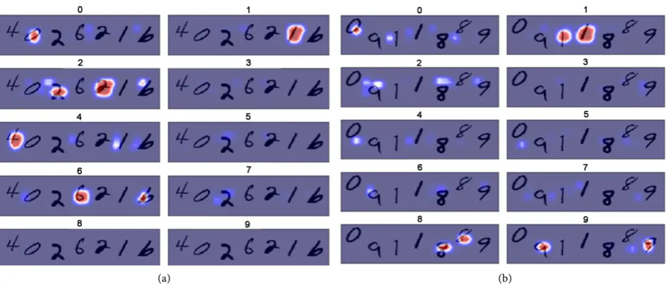
For the multi-digit classification, we show in Figure 5 the response of each digit detector at different locations of the sample input. The redder a region is, the more confident the classifier predicts that digit at that image patch. It can be seen that at correct digit locations, the detector shows consistently confident predictions throughout the region. This can be used to identify a region as con-taining a digit.
We also show in Figure 6 the confidence score that we computed. Redder color indicates presence of a digit. The location where the confidence score is high corresponds very well to where digits are present.
4. Conclusions
This paper applies deep networks to digit classification. Instead of hand designed features, we automatically learn them with a deep network and the back-propagation algorithm. We use a convolutional neural network with ReLU activations. In ad-dition, we use pooling layers to remove unnecessary detail and learn higher level features.
We train our network with stochastic gradient descent. Training progresses quickly, we are able to achieve 90% accuracy with only 1000 iterations. After 100 k iterations, we achieve test performance of 99.3% on the MNIST dataset.
We also study multi-digit classification and propose a method to detect digits in an image with multiple digits. We utilize the fact that our classifier produces a probability distribution. We observe that when the input contains a digit, the classifier produces a distribution with low entropy and high confidence on
Figure 4. Training Curve. On the x-axis we plot the number of training iterations in log scale. On the y-axis we plot the classification accuracy on the test set. It can be observed that accuracy improves very quickly initially, reaching approx-imately 90% accuracy with only 1000 iterations. After that accuracy improves slowly. Eventually we reach an accuracy of 99.3% on the test set.
[image:8.595.62.534.333.535.2](a) (b)
Figure 5. Detection of Multiple Images. Left and right are two examples where our model is able to localize the digits in an image with multiple digits at random positions. We apply our classifier to each patch of the image, and the output of each classification label. Redder color corresponds to higher confidence of the presence of that digit, and blue corresponds to low confidence.
Figure 6. Confidence score indicate the present of a digit. The score is higher (redder) where there is a digit and lower (bluer) when there is not.
[image:8.595.169.428.609.673.2]the correct label. On the other hand, when the input does not contain a digit, the classifier produces an almost uniform distribution. We use this different to detect whether an image patch contains an image. We experiment on multiple digit detection and our method is able to successfully localize digits and classify them.
Future work should further improve accuracy and handle different size of di-gits in the multi-digit detection task.
References
[1] Neumann, L. and Matas, J. (2012) Real-Time Scene Text Localization and Recogni-tion. IEEE Conference on Computer Vision and Pattern Recognition (CVPR), Providence, RI, 16-21 June 2012, 3538-3545.
[2] Neumann, L. and Matas, J. (2010) A Method for Text Localization and Recognition in Real-World Images. Asian Conference on Computer Vision, Springer, Berlin, Heidelberg, 770-783.
[3] Toselli, A.H., Romero, V., Pastor, M. and Vidal, E. (2010) Multimodal Interactive Transcription of Text Images. Pattern Recognition, 43, 1814-1825.
https://doi.org/10.1016/j.patcog.2009.11.019
[4] Bušta, M., Neumann, L. and Matas, J. (2017) Deep Textspotter: An End-to-End Trainable Scene Text Localization and Recognition Framework. IEEE International Conference on Computer Vision (ICCV), Venice, 22-29 October 2017, 2223-2231. [5] Raus, M. and Kreft, L. (1995) Reading Car License Plates by the Use of Artificial
Neural Networks. Proceedings of the 38th Midwest Symposium on Circuits and Systems, 1, 538-541.
[6] Barroso, J., Dagless, E.L., Rafael, A. and Bulas-Cruz, J. (1997) Number Plate Reading Using Computer Vision. Proceedings of the IEEE International Symposium on In-dustrial Electronics, Guimaraes, 7-11 July 1997, 761-766.
[7] Lee, S., Son, K., Kim, H. and Park, J. (2017) Car Plate Recognition Based on CNN Using Embedded System with GPU. 10th International Conference on Human Sys-tem Interactions (HSI), Ulsan, 17-19 July 2017, 239-241.
[8] Al-Hmouz, R. and Challa, S. (2010) License Plate Localization Based on a Probabil-istic Model. Machine Vision and Applications, 21, 319-330.
https://doi.org/10.1007/s00138-008-0164-9
[9] Cun, Y.L., Bottou, L. and Bengio, Y. (1997) Reading Checks with Multilayer Graph Transformer Networks. IEEE International Conference on Acoustics, Speech, and Signal Processing, ICASSP-97, 1, 151–154.
[10] Kamal, N., McCallum, A.K., Thrun, S. and Mitchell, T. (2000) Text Classification from Labeled and Unlabeled Documents using EM. Machine Learning, 39, 103-134.
https://doi.org/10.1023/A:1007692713085
[11] Netzer, Y., Wang, T., Coates, A., Bissacco, A., Wu, B. and Ng, A.Y. (2011) Reading Digits in Natural Images with Unsupervised Feature Learning. NIPS Workshop on Deep Learning and Unsupervised Feature Learning, Granada, 12-17 December 2011, 5.
[12] Maldonado-Bascón, S., Lafuente-Arroyo, S., Gil-Jimenez, P., Gómez-Moreno, H. and López-Ferreras, F. (2007) Road-Sign Detection and Recognition Based on Sup-port Vector Machines. IEEE Transactions on Intelligent Transportation Systems, 8, 264-278.https://doi.org/10.1109/TITS.2007.895311
[13] Forsyth, D.A. and Ponce, J. (2002) Computer Vision: A Modern Approach. Prentice Hall Professional Technical Reference.
[14] Mundy, J.L. and Zisserman, A. (1992) Geometric Invariance in Computer Vision. Vol. 92, MIT Press, Cambridge.
[15] Ke, Y. and Sukthankar, R. (2004) PCA-SIFT: A More Distinctive Representation for Local Image Descriptors. Proceedings of the 2004 IEEE Computer Society Confe-rence on Computer Vision and Pattern Recognition, 27 June-2 July 2004, Vol. 2, 2. [16] Rublee, E., Rabaud, V., Konolige, K. and Bradski, G. (2011) ORB: An Efficient
Al-ternative to SIFT or SURF. IEEE International Conference on Computer Vision, Barcelona, 6-13 November 2011, 2564-2571.
[17] Liu, C., Yuen, J. and Torralba, A. (2016) Sift Flow: Dense Correspondence across Scenes and Its Applications. In: Dense Image Correspondences for Computer Vi-sion, Springer, Cham, 15-49.https://doi.org/10.1007/978-3-319-23048-1_2
[18] Yann, L., Cortes, C. and Burges, C.J.C. (2010) Mnist Handwritten Digit Database.
http://yann.lecun.com/exdb/mnist
[19] Rumelhart, D.E., Hinton, G.E., Williams, R.J., et al. (1988) Learning Representa-tions by Back-Propagating Errors. Cognitive Modeling, 5, 1.
[20] Yann, L., Bengio, Y. and Hinton, G. (2015) Deep Learning. Nature, 521, 436-444.
https://doi.org/10.1038/nature14539
[21] Schmidhuber, J. (2015) Deep Learning in Neural Networks: An Overview. Neural Networks, 61, 85-117.https://doi.org/10.1016/j.neunet.2014.09.003
[22] Nair, V. and Hinton, G.E. (2010) Rectified Linear Units Improve Restricted Boltzmann Machines. Proceedings of the 27th International Conference on Ma-chine Learning, Haifa, 21 June 2010, 807-814.
[23] Yann, L., Boser, B.E., Denker, J.S., Henderson, D., Howard, R.E., Hubbard, W.E. and Jackel, L.D. (1990) Handwritten Digit Recognition with a Back-Propagation Network. Advances in Neural Information Processing Systems, 2, 396-404.
[24] Krizhevsky, A., Sutskever, I. and Hinton, G.E. (2012) ImageNet Classification with Deep Convolutional Neural Networks. Proceedings of the 25th International Con-ference on Neural Information Processing Systems, Lake Tahoe, 3-6 December 2012, 1097-1105.
[25] Lawrence, S., Lee Giles, C., Tsoi, A.C. and Back, A.D. (1997) Face Recognition: A Convolutional Neural-Network Approach. IEEE Transactions on Neural Networks, 8, 98-113.https://doi.org/10.1109/72.554195
[26] LeCun, Y., Jackel, L.D., Bottou, L., Cortes, C., Denker, J.S., Drucker, H., Guyon, I., et al. (1995) Learning Algorithms for Classification: A Comparison on Handwritten Digit Recognition.In: Oh, J.H., Kwon, C. and Cho, S., Eds., Neural Networks: The Statistical Mechanics Perspective, World Scientific, Singapore, 261-276.
[27] Martín, A., Agarwal, A., Barham, P., Brevdo, E., Chen, Z., Citro, C., Corrado, G.S., Davis, A., Dean, J., Devin, M., et al. (2016) Tensorflow: Large-Scale Machine Learning on Heterogeneous Distributed Systems.
[28] Kingma, D.P. and Ba, J. (2014) Adam: A Method for Stochastic Optimization.