Algorithms for Tracking Moving Targets: A Review

Algorithms for Tracking Moving Targets: A Review

Marcelo Queiroz de Lima Brilhante

Pedro Felipe Teixeira Sousa

Auzuir Ripardo de Alexandria

Instituto Federal de Educac¸˜ao, Ciˆencia e Tecnologia do Cear´a - IFCE Campus de Fortaleza

Fortaleza - Cear´a - Brasil

ABSTRACT

Currently there is a huge variety of methods that have been de-veloped to determine the location of a moving object using di-gital image. Multiple approaches have been proposed in the field of computational vision such as: obtaining parameters of position and velocity of an object over time; following suspicious peo-ple in a given environment; automating the collection of infor-mation of vehicle plates; moving a camera to automatically fol-low a ball in a soccer match; or deciding whether a product on a production line in the industry is within the quality standards. This article compiles a brief summary of four techniques related to tracking objects in digital videos. The objective of this work is to present some of the main methods developed so far, show the general structure of the algorithm, address the mathematical fun-damentals and their characteristics, and list the important papers and applications that use them. The review is based on some of the work and theory of methods performed so far. The progress made so far and the main challenges still unresolved will also be eval-uated. Among the several studies, was observed that the various techniques can be used in various combinations to solve a given problem in computer vision, thus mastering such topics is essen-tial for the development of technology in computer vision systems.

General Terms

Algorithm, Computer Vision

Keywords

visual tracking, visual machine, surveillance

1. INTRODUCTION

Tracking an object in a sequence of digital images showing high accuracy in determining motion and positioning is a challenging and comprehensive problem in computer vision. In the develop-ment of algorithms in this field each situation is unique and good solutions require multiple interactions of methods. In this paper, four methods are discussed. The algorithms of the article have for-mulations represented by different functions and equations ranging from the calculation of the center of mass of a binary image to ap-plication of filter based on Fourier transform, least squares method and cross correlation. The objective is to review the mathematical formulation, covering the generalized basic equations, which are

the basis for programming such algorithms. The correct choice of method is crucial in the development and success of any project in-volving real-world applied computer vision. Therefore, some char-acteristics of the method make it appropriate to solve a certain type of problem. One way to track the movement of a given object is to locate it in the video by applying object recognition techniques to each frame, which will be covered in the definition of the char-acteristic to be traced. For example, one can mention its colors, its histogram, its form, the movement it performs, its texture and oth-ers. More specifically in defense, security and enforcement, sev-eral methods have been studied and improved. These characteris-tics give the methods strengths and weaknesses. There are basically three steps in video analysis: detecting a moving object, following the object frame-by-frame and analyzing the object to recognize its behavior. In its simplest form, tracking can be defined as the prob-lem of estimating the trajectory of an object in the plane of the digi-tal image as it moves around the scene. In other words, the crawler assigns a consistent label to the object in the different frames of the video.

[1] highlight, in their article, that object tracking is pertinent in the following computational vision tasks:

—behavior based recognition, that is, human identification based on gait, automatic detection of objects [2];

—automatic surveillance, that is, monitoring the scenario to detect suspicious activity or unwanted events [3];

—videos indexing, i.e. automatic annotations and retrieval of videos in a multimedia database [4];

—Human-computer interaction, that is, gesture recognition, direc-tion of the look for data entry [5];

—Traffic monitoring, that is, collecting real-time data of traffic statistics to direct the flow of cars [6];

—Vehicle navigation, i.e., video-based trajectory planning and the ability to avoid obstacles [7].

[8] state that a strategy commonly used to minimize the com-putational requirement of the vision algorithms is the segmenta-tion and tracking of parameters in the image based on regions-of-interest (ROI). Another technique that is widely used is image sub-sampling. While these techniques are software-oriented, an-other possible approach is to develop special hardware architec-tures, such as dedicated or specific application circuits, and paral-lel processing systems. In short, the tracking algorithms show and highlight objects of interest in a sequence of images, so that, math-ematically, the position parameters of the object relative to the 2D image matrix are determined. Trace methods can be applied in a va-riety of areas, ranging from security / surveillance systems to use in human-machine interface systems. This work presents an approach of the main methods.

2. METHODOLOGY

The methods and techniques applied in solving a computer vision problem, specifically related to tracking, have been constantly im-proved and studied. However, the choice of a specific technique to solve a problem can be a complicated task due to the amount of algorithms for the same purpose.

Initially, was looked at examples of real applications involving computer vision on the Matlab and OpenCV programming lan-guage websites. In the website of the OpenCV library, specifically in the area of ”interesting computer vision algorithms and frame-works”, was analyzed at algorithms that influenced the study of the background subtraction method. Other algorithms were selected based on the computer vision toolbox widely used for computer vi-sion programming in Matlab: KLT, medium change, model match-ing.

Therefore, this article will address the main and most common techniques used by researchers. After a state-of-the-art study on the topic, the research focus is defined in four methods widely used and recurrent in various applications in computer vision. The interest in this subject is due to the high amount of information to solve a cer-tain problem involving computer vision. The importance of this ar-ticle lies in the conclusion of the primordial qualities for a tracking system to function properly through a summary table. This helps in abstraction and develops a broader understanding of the techniques, which are important for programmers. After choosing the common techniques of tracking in computer vision, the research of articles on the subject grounded the theoretical basis of the algorithms and formed the selection of practical examples. Research tools specific to scientific articles were used, such as: researchgate, ACM, IEEE Xplore, CiteSeerX, Robotics and Autonnomous system.

3. THEORETICAL BACKGROUND

Computer vision is the field of computer science that studies the extraction of information from an image. It is intended to program a computer to understand the scene or extract points of interest from the image. The extracted features are used to track the object of interest. Images can be generated by different types of sensors that result in thermal vision, night vision, underwater vision or the imitation of biological vision. For programming, it is necessary to master the tracing algorithms. In this work, was study at the basic fundamentals of the following algorithms: background subtraction; mean shift; KLT; template matching.

In a vision system project, it is important to establish the character-istics of the target and the tracker. The qualitative charactercharacter-istics of a tracker are: number of targets traced, manipulation of occlusions, movement of the target and trajectory of the target. Targets may be

unique (only one target to be traced) or multiple (more than one tar-get). Occlusions are divided into partial or total, or still the inabil-ity to manipulate the occlusion. The movements of the targets are: transverse, scalar, rotation and . The trajectory can be short (when the target is near the image sensor) or long (when the crawler object is far from the camera).

3.1 Extraction of image characteristics

The relationship between detecting and tracking a target is closely linked and in some cases confused. Detecting is extracting the char-acteristics needed for tracing.

According to [9] ), in order to proceed to the project of visual track-ing system, it is important to analyze some factors that are determi-nant in the choice of method and, consequently, to the success of the tracking. Stand out:

—characteristics that best distinguish the target from the environ-ment such as color, appearance and format. Usually one does not have an exact answer, but a good approximation can be decisive for the success of the project;

—conditions to which the object is susceptible during the process. For example, the conditions of luminosity, variation of posture of the target or camera, as well as the dynamics that govern these changes;

—information about the object, which can be assumed a priori. For example, concerning its 3D structure or on whether its recon-struction / learning is possible;

—knowledge of the type of information and frequency of feeding of this system is necessary to achieve the required performance.

A solution widely used by developers is to define a region of in-terest. Given a sequence of images, a mobile element may not be successfully tracked depending on how fast each image is obtained since acquisition and processing obey a certain frequency. If this rate is high enough, the variation of the element position between two consecutive images is not very high. In this case, the tracking does not need to be performed over the entire image; instead, only one region is enough, which contains the target, close to the last de-termined position. Another possible alternative to making tracking faster is to resample the images to smaller resolutions. In this way, as the size of the image decreases, the search space also decreases, although, on the other hand, the level of detail also decreases. Thus, the ideal image size to be used should be carefully analyzed. An-other solution is to invest in more sophisticated equipment, includ-ing, for example, dedicated systems, systems of specific application or parallel architectures [10].

3.2 Background subtraction

previous imagei(t−1)and defining a threshold when transforming to binary image, these edges should be evident since there are few pixels significantly different from zero.

Despite some differences, background subtraction techniques share the same mathematical basis: they are based on the hypothesis that the observed sequence video is made up of a fixed background and the moving object is observed in a plane closer to the camera. In [11] the algorithm is described as follows: assuming that the object has at time t the color (or a color distribution) different from that observed in the background, the principle of the method can be summarized by the following formula:

xt(s)=

1 se d(Is,tBs> τ)

0 se d(Is,tBs≤τ)

(1)

wherext(s)is the motion field of the object at timet(also called

motion mask),dis the distance between the i-th frame of the video at timetin the pixel s andBsis the background in the pixel s;τ

is the threshold. The main differences concerning the techniques are the way B is modeled and how the metric distancedis being used. The easiest way to model background B is with grayscale. The image can be a photo obtained without the presence of the moving object or estimated through a medium temporal filter. In order to obtain an updated background, it can be iteratively updated as follows:

Bs,t+1= (1−α)Bs,t+α·Is,t (2)

Whereαis an update constant ranging from 0 to 1. The foreground pixels, which are the pixels that remain after the subtraction is ap-plied, can be detected by limiting distances such as the three forms below:

d0=|Is,t−Bs,t| (3)

d1=I_s,tR −B_s,tR +

I_s,tG −B_s,tG +

I_s,tB −B_s,tB

(4)

d2= Is,tR −Bs,tR

2

+ IG

s,t−BGs,t

2

+ IB

s,t−BBs,t

(5)

where the exponents R, G and B mean the red, green and blue channels, respectively. Among the techniques for modeling the background, was can at mention the 1-Gaussian, mixed gaussian model, kernel density estimation, maximum minimum and maxi-mum inter-frame difference.

One article that can be cited as an example of this application in practice is [12], which applies the algorithm to detect a pedestrian in the street. The authors use the mixed gaussian model method. In Fig.1, the result is shown at different times, showing the effective-ness of the method.

Once the regions have been identified, the properties of the region become the input for high-level procedures, such as tracing. [13] report that the simplest property is the area A and the centroid (r¯,c¯). Assuming the pixel in square form, the properties are defined as: Area:

A=X

r,c

(6)

Centroid:

¯

r= 1

A · X

r,c

r (7)

Fig. 1. Detection of pedestrian. a) and d) shows the box that delimitates the object, calculated by the algorithm; b) and e) show the result of background subtraction; c) and f) show the result with removal of shadow [11]

¯

c= 1

A · X

r,c

c (8)

Whereris the row andcis the column in the matrix of the image. Andr¯andc¯are respectively the row and column of the calculated centroid. From the coordinates of the centroid, the tracking is then performed. The centroid is then the ’mean’ of the pixel location in the R region. Note that even though each(r, c)belonging to R is a pair of integers,(¯r,c¯)is not usually a pair of integers. Generally an accuracy of more than ten pixels is justifiable for the centroid. [14] present an equation for obtaining the center of mass of an ob-ject from the moment of the image. An image can be represented by a function f that provides the bits 0 or 1 of the image at the coor-dinate point (x, y). Thus, for a 2D image, the ordering moment (p + q) is defined as:

mp,q= nxny

X

1

xpypf(x, y) (9)

Wherenxandnyare respectively the height and the width of the

image.

From the moments previously presented, it is possible to obtain a great amount of both geometric and statistics information of the image. The center of mass can be calculated as follows:

xc= m10

m00 (10)

yc= m01

m00 (11)

Wherexcandycare the centroid coordinates,m00represents the

area of the object of interest, andm01andm10m01 represent the projections of the points of interest on the X and Y axes. An exam-ple of the center of mass calculation is shown in Fig.2.

3.3 Camshift tracking

Fig. 2. Example of calculation of center of mass [14]

given much visibility until applied in the computational view. It is a non-parametric procedure for the estimation of probability den-sity functions widely applied to pattern recognition problems. Its effectiveness in performing high-level visualization tasks, such as tracking, has been explored in a large number of works [17]. In order to segment the image into regions of similar color, mean shift estimates for each pixel the pixel density gradient of similarly colored pixels. The estimates are used, through an iterative proce-dure, to find local density peaks, and all pixels leading to the same peak are taken as part of the same segment [18].

Before the procedure starts, was must at define, for each pixel, its influence window, called kernel, or search window. The kernel de-fines an intuitive measure of the distance between pixels, both spa-tially and in terms of color; their size and shape may have a signif-icant impact on the effectiveness of segmentation [17]

[16] show the basis for the algorithm mathematically. Given a sam-ple S=si,siRand a kernel K, the main sample using K at point x:

m(x) =

P

isiK(si−x)

P

iK(si−x)

(12)

Where k is the uniform kernel given by:

K(x) =

1 sekxk ≤λ

0 sekxk> λ

(13)

k can also be represented by normal kernel:

K(x) =c.exp

−1

2kxk

2

(14)

The differencem(x)−xis called mean shift. The repeated move-ment of the data points for the main sample is called the mean shift algorithm. At each iteration of the algorithm,s ← m(s)is done for all sS simultaneously [19].

[20] describe the main properties of camshift:

—automatic speed convergence - vector size depends on the gradi-ent;

—convergence is only guaranteed for infinitesimal iterations; —for a uniform kernel, convergence is achieved in a finite number

of iterations;

—normal (Gaussian) kenel exhibits a smooth trajectory but it is slower.

Camshift (Continuously Adaptive Mean-SHIFT) is an algorithm developed for color tracking, thus enabling face tracking. It is based on a statistical technique where the peak is sought between distri-butions of probability in density gradients. This technique is called ”mean shift” and has been adapted in Camshift to address the dy-namic change of color probability distributions in a video sequence. It can be used in object tracking and face tracking [21].

The goal of Camshift is simple. Through a set of points (projection of histograms), a small window of an image is selected. The algo-rithm moves the small window to a maximum area of pixel density [21].

The start window shows the blue circle namedC1. Its center is marked with a blue rectangle,C10. But if the centroid of the points

is found inside that window, then the pointC1ris the real centroid

of the window. Then the window moves so that the circle of the new window matches the previous centroid. It does another itera-tion and continues until the center of the window and its centroid are in the same location. Finally, was have at window with the max-imum distribution of pixels as seen in Fig.3.

For each frame, the raw image is converted to another color proba-bility distribution through a skin color histogram model. The center and size of the face to be tracked are found through the CamShift operating on the color probability image. The current face size and location are informed and used to set the size and location of the search window for the next video image.

Fig. 3. Pixel distribution [22]

3.4 KLT Tracking

The acronym KLT refers to Kanade-Lucas-Tomasi. In their three works: [23]; [24]; [25], they developed a tracing method based on feature extraction.

It is an algorithm based on features such as borders, points, con-tours, shapes or textures. For the optimal performance of this algo-rithm, it is necessary to define the ideal characteristics of the object of interest.

Some of the feature tracking algorithms are: harris conner, sobel, viola-jones. The algorithm tracks the characteristic points of the tar-get. In addition to the mentioned algorithms, the points of interest can be generated by the ”good features to track” method proposed by [23]

KLT uses spatial intensity information to direct the search for the position that reaches the best combination. This algorithm is faster than traditional techniques that examine potential combinations be-tween images, such as template matching [23].

An important problem in finding a D-shift from one point to the next in a frame is that was cannot at follow a single pixel, unless it has a brightness very different from its neighborhood. In fact, the pixel value may change due to noise and then be confused with its adjacent ones. As a consequence, it is difficult or even impossible to determine where the pixel is in the next frame based only on local information. Due to these problems, not followed by a single pixel, but a pixel window.

This method is based on the translational image registration prob-lem which is characterized as follows:

—calculate the translation motion between consecutive frames; —attach the motion vectors in successive frames to get the track

for each point;

—introduce new feature calculation by applying the desired algo-rithm to every 10 or 15 frames;

—follow new and old points using steps 1-3.

[23] describe the algorithm in their work: KLT algorithm is based on three hypotheses: (1) constant brightness, the brightness of the tracked pixel does not change; (2) continuous time or limited move-ments by the target between consecutive frames; (3) consistent space, within a small space w the motion vector remains constant or the target followed maintains a similar motion. The KLT algo-rithm is based on the gray scale metric SSD (sum of the square of the difference) of the trace window w. This is:

=

Z·

w

J

X+d 2

−IX+x

d

2

w(x)dx (15)

WhereJ is the current frame;I is the previous frame; X is the matrix of the image. Although the KLT algorithm has advantages regarding speed and precision, it also has several drawbacks, such as: (1) when the displacementdis too long, the KLT may lose track of the target and float; (2) KLT requires a constant brightness, so when there is noise interference, the margin of error is increased, then equation 15 is not equal to or near zero, thus affecting target tracking; in addition to that, inconstant brightness often occurs in the real world, which makes the system poor in robustness; (3) the characteristic points may result in error in the task of following due to blockage or changes in target shape. In the example illustrated below was can at see that points 1 and 2 are used as points to be followed, and while the algorithm manages to trace point 1, it loses point 2.

KLT is also a tracking algorithm that uses optical flow method, which makes it accurate and reactive. In this technique it assumes that the flow is essentially constant in a neighborhood of the consid-ered pixel and solves the basic optical flow equation for all neigh-boring pixels. When it is applied to a small window and when the magnitude of movement is significant, the crawler fails [25] The main components of any feature tracker are accuracy and ro-bustness. The accuracy component relates the local sub-pixel as-signed to the trace, that is, the label that follows the target over time. Intuitively, a small integration window is preferred in order not to ’undo’ the details contained in the image, for example small values ofw(x). This is especially necessary in areas where oc-clusions occur and where two segments move at different speeds. Robustness relates to tracking sensitivity with regard to changes in illumination, image size in motion. In particular, in order to han-dle large displacements, a wide integration window is preferable. In fact, considering equation 15, it is preferable to have d

2 less

than window w. There is therefore an intrinsic relationship between accuracy and robustness when choosing the size of the integration window [26].

3.5 Template matching tracking

Different matching strategies have been proposed in the literature to solve issues involving tracking.

[27] defines matching as the purpose of detecting the variation in the position of a point between two images using a matching stage, that is, finding the same point in two different images.

Template matching is a method of searching and finding the loca-tion of a template in a larger image. The correlaloca-tion can be basically

understood as the matching of points of interest in different frames. There are some functions to perform this task.

[28] propose the cross-correlation technique, in which the template is moved through the input image (as in a 2D convolution) and then the template is compared with pieces of the input image. The result is a grayscale image where each pixel denotes how closely the neighborhood of that pixel matches. Mathematically it has been:

cf,g=

X

[i,jR]

f(i, j)g(i, j) (16)

The variance normalized correlation (VNC) is the function com-monly used in correlation [28]. This technique has the advantage of providing stable and reliable results even in a wide variety of en-vironments. The fact that the VNC is normalized has an advantage over other correlation functions because the choice of the threshold becomes easier.

The correlation between two points of two images is given by [29]:

V N Cp, p0=

Pk i,i0

I(i)−I¯p0.I0i0−I¯0p0

nq_σ2 1.σ₁20

(17)

whereKis the correlation neighborhood window, and,N is the number of pixels in the neighborhood, andσ2

1I¯are the variance and

the average of intensity in the neighborhood, respectively. There-fore, the performance of the algorithm basically depends on two parameters: window size and neighborhood.

Correlation Filter-based trackers (CTFs) have drawn attention in the field of object tracking due to recently noticeable advances. It was first published in 2010, so it is more recent than other algo-rithms. There are several techniques using this approach, such as: Average of Synthetic Exact Filters (ASEF), Unconstrained Mini-mal Average Correlation Energy (UMACE), and Minimum Output Sum of Squared Error (MOSSE).

[30] summarize the basic structure: initially, the correlation filter is trained with a cropped piece of the image at a certain target position in the first frame. At each subsequent step, a fragment of the pre-dicted position is then cut off for use in detection. Then, as shown in Fig.4, various features can be extracted from the raw input data, and a cosine-generated window is generally applied to smooth the effects of the edges. Subsequently, correlation operations are per-formed by substituting convolutions with element-by-element mul-tiplications using the discrete Fourier transform. Following the cor-relation procedure, a spatial map or response map can be obtained using the inverse transform. The position with the maximum value in this map is assumed to be the new state of the target. Then what appears in the estimated position is extracted to train and update the correlational filter. To describe the process mathematically, assume that x is the input at the detection stage, and h is the correlation filter. In practice, x may be a piece of the raw image or a repre-sentation of the characteristic. Suppose that the hat element is the Fourier transform of a vector. According to the convolution theo-rem, cyclic convolution equals element-to-element multiplication in the frequency domain [31].

x⊗h==−1xˆ⊗hˆ (18)

Onde=−1

Where=−1

Fig. 4. General flow chart for a typical tracking method based on correlational filter [30]

map. To train the filter, was first as define the output correlation as

y. Using the newx0 instance of the target, the correlation filterh

must satisfy

y==−1xˆ0ˆh (19)

ˆ

h= yˆ ˆ

x0 (20)

Whereyˆis the transform ofy, and the division is made element by element.

There are some demands for the algorithm efficiency. Firstly, the training scheme is crucial for the CTF algorithm. Since the target can constantly change its appearance, correlation filters must be trained to adapt and update themselves on-the-fly to adapt to the new appearance of the target. Secondly, the different methods that represent the target’s characteristic are a major performance influ-encer. Although raw pixels can be used for detection, the crawler may be affected by various noises such as light changes and blur generated by the movement. Representations of more powerful fea-tures may help a lot.

4. RESULTS

A good tracker accomplishes the task of tracking with reliability, precision and robustness. However, evaluating crawlers is difficult because a number of factors can affect the performance of track-ing the object. [32] describe the attributes that can affect perfor-mance: light variation, scale variation, occlusion, deformation, mo-tion spots, speed of movement, rotamo-tion and low resolumo-tion. In addi-tion, different quantitative metrics are used in the articles analyzed, such as precision, recall, frames rates, which makes it difficult to define a universal and common metric for all. In addition to that, in all performance evaluations, authors use video datasets, widely used and accepted in the academic community, for example VIVID, CAVIAR, and PETS, TDL where the algorithms are tested exten-sively in different everyday situations, which is outside the scope

of this work, so the quantitative evaluation will not be discussed here. Therefore this paper focuses on qualitative terms, which are usual in tracking tasks. As skills, has been listed: single or multiple objects, manipulating occlusion, long and short-term trajectories, types of target movement: transverse, scale, rotation, homographic [33, 34, 32, 35].

[12] perform the tracing by applying backgoround subtraction to follow two moving objects, being able to differentiate one object from the other. In the work of [36], they show the example of using the camshift algorithm to successfully track an object that moves in the direction of translation and undergoes change in scale and occlusion. [22] show an innovative application of camshift, which uses multiple target characteristics to resolve interferences and par-tial occlusions. [37] present a precise crawler using feature extrac-tion in the frontier of objects, demonstrating complex target move-ment and tracking success. [37] compare several template-based algorithms and show an example of rotation tracking that is well resolved by the method.

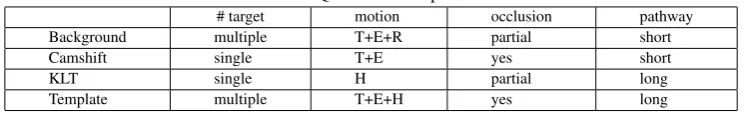
Table 1 summarizes the strengths of each tracker, which can be useful in choosing an algorithm for a specific task. The long-term trajectory can be understood as a more complex task, with different occlusions, varied changes from the point of view of the camera. Usually a highly complex trajectory,[38], it can be seen as a trajec-tory difficult to trace. The short-term is a trajectrajec-tory in structured environments, with previously limited movements and the target occupies a large space of the image. This table is neither perma-nent or unchanged, as long as the techniques are changed and get better.

5. DISCUSSION

Table 1. Qualitative comparison.

# target motion occlusion pathway

Background multiple T+E+R partial short

Camshift single T+E yes short

KLT single H partial long

Template multiple T+E+H yes long

and computational tracking, and in some cases the methods can be applied together for robustness.

[1] create groups in the tasks related to tracing to facilitate the mat-uration of the subject. That helps in understanding, but it is not definitive, because in some applications the groups of the created taxonomy interact, which makes it difficult to separate them and group them together. In the background-based tracking technique, [39] deal with a robust application in a real-world scenario, demon-strating the effectiveness of the method and its evolution in over-coming its weaknesses such as fixed background and highly struc-tured environment. The histogram-based method tends to fail when occlusions occur or when there is color interference. To solve this problem, [40] and [36] use the Kalman filter as an aid to obtain satisfactory results.

KLT is believed to be good for tracking faces, as shown by [41]. In the template-based algorithm, was can analyze some limitations and disadvantages that sometimes do not make it applicable in prac-tical situations. This method assumes that the appearance of the object is constant or varies little from frame to frame. However, [42], show that the correlation algorithm using adaptive filters can be very fast due to its simplicity, reaching to process at 669 fps in a tracking application.

Several techniques and methods are not addressed in this work, such as motion estimators, optical flow and predictors such as the Kalmam filter.

6. CONCLUSION

In this article, a summary of the object tracking techniques was presented and a brief review of related topics was reported. We summarized the main object trackers and the generalization of their basic principles, and a table was presented listing the strengths of the crawlers discussed in the article. Although the object track-ing is a well established problem in computer vision cite comani-ciu2003kernel, isard1998icondensation, jepson2003robust, supan-cic2013self, it still remains a challenging task. The summary of tracking techniques aids in intuitive insight into this important topic of machine vision research. The contribution of this work to the field of computer vision is important, since it generalizes a basic approach of the main algorithms. Although it is a well explored subject, it is still challenging and the practical application of this technology is already a reality. It can be said that there are still great opportunities for exploitation by mechatronics technology, for ex-ample, by combining control systems and image sensors. The sum-mary of tracking techniques aids in intuitive insight into this im-portant topic of machine vision research.

7. REFERENCES

[1] Alper Yilmaz, Omar Javed, and Mubarak Shah. Object track-ing: A survey. Acm computing surveys (CSUR), 38(4):13, 2006.

[2] Jake K Aggarwal and Quin Cai. Human motion analysis: A review. InNonrigid and Articulated Motion Workshop, 1997. Proceedings., IEEE, pages 90–102. IEEE, 1997.

[3] Ahmed Elgammal, Ramani Duraiswami, David Harwood, and Larry S Davis. Background and foreground model-ing usmodel-ing nonparametric kernel density estimation for visual surveillance. Proceedings of the IEEE, 90(7):1151–1163, 2002.

[4] Michal Irani and Prabu Anandan. Video indexing based on mosaic representations.Proceedings of the IEEE, 86(5):905– 921, 1998.

[5] Manuel Jes´us Mar´ın-Jim´enez, Andrew Zisserman, Marcin Eichner, and Vittorio Ferrari. Detecting people looking at each other in videos. International Journal of Computer Vi-sion, 106(3):282–296, 2014.

[6] Pooja Kudav and Pranav Acharya. Automated traffic control system using big data and cognitive analysis. International Journal of Computer Applications, 151(10), 2016.

[7] Victor Vaquero, Ely Repiso, Alberto Sanfeliu, John Vissers, and Maurice Kwakkernaat. Low cost, robust and real time system for detecting and tracking moving objects to auto-mate cargo handling in port terminals. InRobot 2015: Second Iberian Robotics Conference, pages 491–502. Springer, 2016. [8] Mansi Manocha and Parminder Kaur. Roi based video object tracking using mean kernel profile of histogram.International Journal of Computer Applications, 3(8), 2014.

[9] Geraldo Silveira, Jos RH CARVALHO, Samuel Siqueira BUENO, and Marconi K MADRID. Uma revisao das tec-nicas de controle servo visual de robos. 2010.

[10] Davi Yoshinobu Kikuchi. Sistema de controle servo visual de uma camera pan-tilt com rastreamento de uma regiao de referencia.PhD thesis, Universidade de Sao Paulo, 2007. [11] Yannick Benezeth, Pierre-Marc Jodoin, Bruno Emile, H´el`ene

Laurent, and Christophe Rosenberger. Review and evalua-tion of commonly-implemented background subtracevalua-tion algo-rithms. InPattern Recognition, 2008. ICPR 2008. 19th Inter-national Conference on, pages 1–4. IEEE, 2008.

[12] Omar Javed and Mubarak Shah. Tracking and object classi-fication for automated surveillance. Computer VisionECCV 2002, pages 439–443, 2006.

[13] L Shapiro and G Stockman. Computer vision, pp prentice-hall.New Jersey, USA, 2001.

[14] Simon Medeiros Soares, Thiago de Castro Turino, Mari-ane Rembold Petraglia, and Jose Gabriel Rodriguez Carneiro Gomes. Rastreamento de objetos utilizando processamento de imagem. 2010.

[15] Maur´ıcio Marengoni and Stringhini Stringhini. Tutorial: Introduc¸˜ao `a vis˜ao computacional usando opencv.Revista de Inform´atica Te´orica e Aplicada, 16(1):125–160, 2009. [16] Keinosuke Fukunaga and Larry Hostetler. The estimation of

[17] Jue Wang, Bo Thiesson, Yingqing Xu, and Michael Cohen. Image and video segmentation by anisotropic kernel mean shift.Computer Vision-ECCV 2004, pages 238–249, 2004. [18] Guilherme Machado Gagliardi et al. Sistema robusto de

acompanhamento de trajetoria de alvos moveis. PhD thesis, UNIVERSIDADE DE S ˜AO PAULO, 2014.

[19] Yizong Cheng. Mean shift, mode seeking, and clustering. IEEE transactions on pattern analysis and machine intelli-gence, 17(8):790–799, 1995.

[20] Dorin Comaniciu and Peter Meer. Mean shift analysis and ap-plications. InComputer Vision, 1999. The Proceedings of the Seventh IEEE International Conference on, volume 2, pages 1197–1203. IEEE, 1999.

[21] Rafael C Gonzalez, Steven L Eddins, and Richard E Woods. Digital Image Publishing Using MATLAB. Prentice Hall, 2004.

[22] Zhiyu Zhou, Dichong Wu, Xiaolong Peng, Zefei Zhu, and Kaikai Luo. Object tracking based on camshift with multi-feature fusion.JSW, 9(1):147–153, 2014.

[23] Jianbo Shi et al. Good features to track. InComputer Vi-sion and Pattern Recognition, 1994. Proceedings CVPR’94., 1994 IEEE Computer Society Conference on, pages 593–600. IEEE, 1994.

[24] Carlo Tomasi and Takeo Kanade. Detection and tracking of point features. 1991.

[25] Bruce D Lucas, Takeo Kanade, et al. An iterative image reg-istration technique with an application to stereo vision. 1981. [26] Jean-Yves Bouguet. Pyramidal implementation of the affine lucas kanade feature tracker description of the algorithm.Intel Corporation, 5(1-10):4, 2001.

[27] Gloria Liliana Lopez Munoz. Analise comparativa das tec-nicas de controle servo-visual de manipuladores roboticos baseadas em posicao e em imagem. 2011.

[28] Etienne Vincent and Robert Laganiere. An empirical study of some feature matching strategies. InProc. Conf. Vision Interface, Calgary, Canada, pages 139–145, 2002.

[29] Henrik Andreasson, Andr´e Treptow, and Tom Duckett. Self-localization in non-stationary environments using omni-directional vision. Robotics and Autonomous Systems, 55(7):541–551, 2007.

[30] Zhe Chen, Zhibin Hong, and Dacheng Tao. An experimen-tal survey on correlation filter-based tracking. arXiv preprint arXiv:1509.05520, 2015.

[31] H. Collewign, C. J. Erkelens, and R. M. Steinman. Binocular co-ordination of human horizontal saccadic eye movements. Journal of Physiology, 404:157–182, oct 1988.

[32] Yi Wu, Jongwoo Lim, and Ming-Hsuan Yang. Online ob-ject tracking: A benchmark. InProceedings of the IEEE con-ference on computer vision and pattern recognition, pages 2411–2418, 2013.

[33] Robert Collins, Xuhui Zhou, and Seng Keat Teh. An open source tracking testbed and evaluation web site. InIEEE In-ternational Workshop on Performance Evaluation of Tracking and Surveillance, volume 35, 2005.

[34] Robert B Fisher. The pets04 surveillance ground-truth data sets. InProc. 6th IEEE international workshop on perfor-mance evaluation of tracking and surveillance, pages 1–5, 2004.

[35] Zdenek Kalal, Krystian Mikolajczyk, and Jiri Matas. Tracking-learning-detection. IEEE transactions on pattern analysis and machine intelligence, 34(7):1409–1422, 2012. [36] Liang Li and Yi Luo. Improved video moving target

track-ing based on camshift. American Journal of Computational Mathematics, 6(04):357, 2016.

[37] Santhosh K Ramakrishnan, Swarna Kamlam Ravindran, and Anurag Mittal. Comal tracking: Tracking points at the object boundaries. arXiv preprint arXiv:1706.02331, 2017. [38] Peter Ochs, Jitendra Malik, and Thomas Brox.

Segmenta-tion of moving objects by long term video analysis. IEEE transactions on pattern analysis and machine intelligence, 36(6):1187–1200, 2014.

[39] Sen-Ching S Cheung and Chandrika Kamath. Robust tech-niques for background subtraction in urban traffic video. In Proceedings of SPIE, volume 5308, pages 881–892, 2004. [40] Zheng Han, Rui Zhang, Linru Wen, Xiaoyi Xie, and

Zhi-jun Li. Moving object tracking method based on improved camshift algorithm. In Industrial Informatics-Computing Technology, Intelligent Technology, Industrial Information In-tegration (ICIICII), 2016 International Conference on, pages 91–95. IEEE, 2016.

[41] Ritesh Boda and Jasmine Pemeena Priyadarsini. Face detec-tion and tracking using klt and viola jones. InARPN, vol-ume 11, pages 13472–13476, 2016.