Improving likelihood ratio based confidence intervals for threshold parameters in finite samples

Aut

omatic

all

yg

ener

at

ed

rough

PDF

by

Pr

oo

fCheck

fr

om

Ri

ver

Valle

yT

ec

hnologies

Lt

d

Luiggi Donayre

_{/ Yunjong Eo}

_{/ James Morley}

Improving likelihood-ratio-based confidence

intervals for threshold parameters in finite

samples

1_{Department of Economics, University of Minnesota–Duluth, 1318 Kirby Dr., Duluth, MN 55812, USA, E-mail:} [email protected]

2_{School of Economics, University of Sydney, Sydney 2006, Australia}

3_{School of Economics, University of New South Wales, Sydney 2052, Australia}

Abstract:

Within the context of threshold regressions, we show that asymptotically-valid likelihood-ratio-based confi-dence intervals for threshold parameters perform poorly in finite samples when the threshold effect is large. A large threshold effect leads to a poor approximation of the profile likelihood in finite samples such that the con-ventional approach to constructing confidence intervals excludes the true threshold parameter value too often, resulting in low coverage rates. We propose a conservative modification to the standard likelihood-ratio-based confidence interval that has coverage rates at least as high as the nominal level, while still being informative in the sense of including relatively few observations of the threshold variable. An application to thresholds for US industrial production growth at a disaggregated level shows the empirical relevance of applying the proposed approach.

Keywords:confidence interval, finite-sample inference, inverted likelihood ratio, threshold regression JEL classification:C13, C20

DOI:10.1515/snde-2016-0084

1 Introduction

Threshold regression models specify that regression functions can be divided into several regimes based on the value of an observed variable, called a threshold variable, related to threshold parameters. Threshold regression models and their various extensions have become standard for the specification of nonlinear relationships be-tween economic variables (see Potter, 1995; Balke, 2000; Koop & Potter, 2004; Gonzalo & Pitarakis, 2013, among many others.).1_{There have been important developments in the asymptotic theory for inference in threshold}

regression models (see Chan, 1993; Hansen, 1996; Chan & Tsay, 1998; Hansen, 2000). However, Enders, Falk, and Siklos (2007) show that when the threshold parameter is unknown, asymptotic and bootstrap approxima-tions of finite sample distribuapproxima-tions do not result in satisfactory confidence intervals (CIs) for slope or threshold parameters in stationary threshold autoregressive models.

In this paper, we are particularly interested in the finite sample performance of asymptotically-valid likelihood-ratio-based CIs for the threshold parameter proposed by Hansen (1997, 2000) . Using Monte Carlo experiments, we show that the performance of the CIs becomes particularly problematic in finite samples when the threshold effect is relatively large. This finding is puzzling because the coverage rates of CIs are expected to converge to a nominal level when the threshold effect increases (i.e. there is more precise information about the true threshold value).

We conjecture that when the threshold effect is large, the approximation of the profile likelihood becomes poor and leads to lower coverage rates of the CIs. As noted above, we would expect large threshold effects to help the CIs achieve accurate coverage rates relative to a nominal level given the benefits in terms of econo-metric identification. However, the large threshold effects could also lead to the discrete approximation of the profile likelihood for the threshold parameter becoming highly imprecise. Thus, a large threshold effect has two conflicting impacts and the performance of the CIs depends on which impact is bigger. When the magnitude of the threshold effect is particularly large, the poor approximation dominates the benefit from the more precise information and the standard CIs perform poorly.

Luiggi Donayreis the corresponding author.

Aut

omatic

all

yg

ener

at

ed

rough

PDF

by

Pr

oo

fCheck

fr

om

Ri

ver

Valle

yT

ec

hnologies

Lt

d

Why does the large threshold effect make the approximation so poor? To construct the CIs, Hansen (2000) inverts the likelihood-ratio test for the threshold parameter by evaluating the profile likelihood at observed threshold values and includes the threshold values for which the likelihood-ratio test cannot be rejected. The asymptotic theory for the likelihood-ratio test is developed under the assumption that the threshold variable is distributed with acontinuousdistribution. However, in finite samples, the threshold variables are observed discretely and the profile likelihood for the test is constructed using a step function approximation for the threshold values that are not observed in the sample. When the threshold effect is small (i.e. there is less infor-mation about the true threshold value), the likelihood-ratio tests for the threshold parameter are rarely rejected and the CIs includes many threshold values. Thus, the step function would approximate the likelihood func-tion effectively when constructing the CIs. However, when the threshold effect is large, the likelihood-ratio tests for the threshold parameters are rejected too often and the CIs include few threshold observations. With few observations, the step function then becomes a poor approximation of the likelihood and the CIs may exclude the true threshold parameter, resulting in low coverage rates, even in large samples.

We consider two possible modifications to Hansen’s inverted likelihood-ratio (ILR) approach in order to

address the step function approximation: (i) an equally-spaced grid-search approach; and, (ii) a conservative approach that extends the CIs to the closest observations excluded by the standard ILR approach. We then conduct Monte Carlo simulations to evaluate the performance of the original ILR approach and the proposed modifications, using two different data-generating processes (DGPs). For each approach, we evaluate the cov-erage rate, avcov-erage length and avcov-erage number of threshold values included in the CIs.

Our results suggest that the standard ILR approach massively undercovers the true threshold parameter when the threshold effect is large, even for sample sizes as large asn = 1,000. This poor performance is ex-plained by the‘sharp’profile likelihood associated with a large threshold effect, which results in too few

pos-sible threshold values being included in the CIs. Thus, the large threshold effect leads to a poor approximation of the profile likelihood in finite samples. The refined grid-search improves the performance by including some of the non-observed, but possible threshold values, but the coverage rates are still far below the nominal level in most cases. Meanwhile, the conservative approach has coverage rates at least as high as the nominal level, while still being informative in the sense of including relatively few observations of the threshold variable.

Based on these Monte Carlo results, we recommend researchers use the conservative approach when structing CIs for threshold parameters in practice. We also confirm the empirical relevance of using the con-servative approach relative to the benchmark approach with an application to thresholds for US industrial production growth at a disaggregated level. Notably, we find that the conservative approach includes the com-monly hypothesized threshold value of zero (e.g., Potter, 1995) in more cases than the benchmark approach.

2 Threshold regressions

We consider a general class of threshold regressions. Following Hansen (2000), regression parameters switch between two regimes according to

𝑦𝑖= 𝜃′1𝑥𝑖+ 𝑒𝑖, 𝑖𝑓 𝑞𝑖 ≤ 𝛾 (1)

𝑦𝑖= 𝜃′2𝑥𝑖+ 𝑒𝑖, 𝑖𝑓 𝑞𝑖 > 𝛾 (2)

fori = 1,…,n, where xi ∈ ℝkis a vector of regressors; the threshold variable qisplits the sample into two

regimes;γis the unknown threshold parameter;y_iis generated by either (1) or (2) depending on the value ofq_i

relative toγ; ande_iis a regression error.2For expositional purposes, the threshold regression model (1)–(2) can

be rewritten in a single-equation form:

𝑦𝑖= 𝜃′𝑥𝑖+ 𝛿′𝑛𝑥𝑖(𝛾) + 𝑒𝑖 (3)

whereθ=θ₂,δ_n= (θ₁−θ₂),x_i(γ) =x_id_i(γ),d_i(γ) =1{q_i≤γ}, and1{⋅} is the indicator function.3

An estimate of γ can be obtained through concentration. Conditional onγ, (3) is linear in θand δ. The

conditional estimatorsθ(γ) andδ(γ) can be found by regressingy= (y₁,…,y_n)′on𝑋∗

𝛾= [𝑋 𝑋𝛾], whereXandXγ are stacking matrices of the vectors𝑥′

𝑖and𝑥𝑖(𝛾)′in equation (3), respectively. As is standard in the literature,γ

is restricted to be in a bounded setΓ= [𝛾, 𝛾]to avoid small-sample distortions. In practice,𝛾and𝛾correspond

Aut

omatic

all

yg

ener

at

ed

rough

PDF

by

Pr

oo

fCheck

fr

om

Ri

ver

Valle

yT

ec

hnologies

Lt

d

Then, the grid-search procedure occurs overΓ𝑛=Γ∩ {𝑞𝑖}𝑛𝑖=1, so that all elements inΓnare simply all observed values ofq_ibetween𝛾and𝛾.

The sum of squared errors function forγis given by

𝑆𝑛(𝛾) = 𝑆𝑛(𝜃(𝛾), 𝛿(𝛾), 𝛾) = 𝑦′𝑦 − 𝑦′𝑋𝛾∗(𝑋∗

′

𝛾𝑋𝛾)−1𝑋∗

′

𝛾𝑦. (4)

and the estimate ofγis given by the value that minimizes (4):

̂

𝛾 =arg min

𝛾∈Γ𝑛 𝑆𝑛(𝛾). (5)

3 Confidence intervals for threshold parameters

3.1 Benchmark ILR approach

Following Hansen (2000), we construct a (1−α) confidence interval forγ by inverting anα-level likelihood

ratio (LR) test of the hypothesis𝐻0 ∶ 𝛾 = 𝛾0. Hansen (2000) shows that the LR statistic under the auxiliary assumption that𝑒𝑖∼ 𝑖𝑖𝑑𝑁(0, 𝜎2)is given by

𝐿𝑅𝑛(𝛾) = 𝑛

𝑆𝑛(𝛾) − 𝑆𝑛( ̂𝛾)

𝑆𝑛( ̂𝛾)

(6)

withSn(γ) defined as in equation (4). It is well known that the distribution of the LR statistic in (6) is

non-standard.

The 1−α ILR confidence set for the threshold parameter consists of all the possible values ofγ∈Γ_nfor which the null hypothesis would not be rejected at theαlevel:

𝐶𝑑= {𝛾 ∶ 𝐿𝑅𝑛(𝛾) ≤ 𝐶𝑉1−𝛼, 𝛾 ∈Γ𝑛} (7)

whereCV1−αis the critical value derived by Hansen (2000). Note that the confidence set in (7) may be disjoint. However, we can construct a convexified confidence interval by connecting all disjoint segments, which we set as thebenchmarkconfidence interval in this paper.

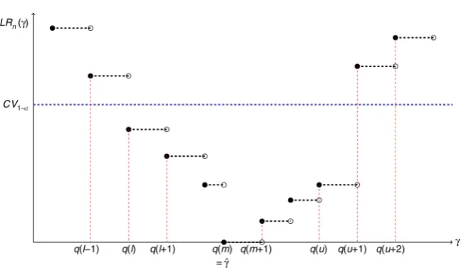
To illustrate the benchmark approach to constructing confidence intervals, we display a hypothetical LR profile in Figure 1. Letq(j) denote thej-th ordered possible threshold value among allq_i∈Γ_n. Suppose thel-th possible threshold valueq(l) and theu-th possible threshold valueq(u) are the boundaries of the ILR confidence interval, defined as the minimum and maximum values in the ILR confidence set (7), respectively:

𝑞(𝑙) =min{𝑞𝑖∶ 𝐿𝑅𝑛(𝑞𝑖) ≤ 𝐶𝑉1−𝛼, 𝑞𝑖∈Γ𝑛} (8)

𝑞(𝑢) =max{𝑞𝑖 ∶ 𝐿𝑅𝑛(𝑞𝑖) ≤ 𝐶𝑉1−𝛼, 𝑞𝑖 ∈Γ𝑛} (9)

Then, the 1−αbenchmark ILR confidence interval is given by

𝐶𝑏= {𝛾 ∶ 𝑞(𝑙) ≤ 𝛾 ≤ 𝑞(𝑢)} (10)

whereq(l) andq(u) are defined in (8) and (9), respectively. See Figure 1.

Theoretically, because the confidence interval is constructed by completing the disjoint segments in (7), the coverage rate of the benchmark interval (10) is expected to be greater than 1−α, at least asymptotically in the

Aut

omatic

all

yg

ener

at

ed

rough

PDF

by

Pr

oo

fCheck

fr

om

Ri

ver

Valle

yT

ec

hnologies

Lt

d

3.2 Conservative ILR approach

The motivation for the conservative modification to the standard ILR approach stems from the fact that we use a step function approximation of the likelihood function for possible values of the threshold that we do not observe (i.e., any points𝛾 ∉ {𝑞𝑖}𝑛𝑖=1) becauseΓnis a collection of discrete observations in the parameter space of Γin finite samples. Specifically, the threshold values betweenq(u) andq(u+ 1) and betweenq(l−1) andq(l) are

excluded in the benchmark confidence interval. However, it is likely that there are some threshold parameter values 𝛾 ∈ (𝑞(𝑢), 𝑞(𝑢 +́ 1))such that 𝐿𝑅𝑛( ́𝛾) ≤ 𝐶𝑅1−𝛼.4 If these values are not included in the confidence

interval, it may exclude the true threshold value and its coverage rate could be far lower than 1−α.

Indeed, the benchmark ILR approach attains unsatisfactory coverage rates when the threshold effect is large. This large threshold effect leads to the‘sharp’empirical LR profile. This implies that a sequence of LR tests for

the possible threshold values are rejected too often, leading to the inclusion of too few sample observations of the threshold variable being included in the benchmark ILR confidence intervals. Then, LR evaluations based on{𝑞𝑖}𝑛𝑖=1 are poor approximations to the profile likelihood for threshold parameter γso that the threshold parameter spaces betweenq(u) andq(u+ 1) and betweenq(l−1) andq(l) become relatively large. The large

spaces betweenq(u) andq(u+ 1) and betweenq(l−1) andq(l) would lead to low coverage rates.5To overcome

this issue, we modify the ILR approach by means of a conservative approach.

Intuitively, the conservative approach accounts for non-observed, but possible threshold values whose LR values are lower than the critical value by extending the benchmark ILR confidence interval to include the possible threshold value smaller than, but closest toq(l) in (8) and the possible threshold value larger than, but closest toq(u) in (9) in a conservative way. Formally,

𝑞(𝑙 −1) =max{𝑞𝑖∶ 𝑞𝑖∈Γ𝑛, 𝑞𝑖 < 𝑞(𝑙)} (11)

𝑞(𝑢 +1) =min{𝑞𝑖∶ 𝑞𝑖∈Γ𝑛, 𝑞𝑖> 𝑞(𝑢)} (12)

forq(l) andq(u) defined in (8) and (9), respectively. Based on Figure 1, thus, we can define the conservative confidence interval as follows:

𝐶𝑐= {𝛾 ∶ 𝑞(𝑙 −1) < 𝛾 < 𝑞(𝑢 +1)} (13)

whereq(l−1) andq(u+ 1) are defined in (11) and (12), respectively. Therefore, the conservative confidence

interval (13) includes all non-observable threshold values betweenq(l−1) andq(l) and betweenq(u) andq(u

+ 1). Notice that, by construction, the conservative confidence interval Cc in (13) is always longer than the

benchmark ILR confidence interval.

3.3 Refined grid-search

In addition to the benchmark and conservative approaches, we consider the refined grid-search over the equally-spaced gridΓ_r =Γ∩ qr where the elements inqr are given by 𝑞𝑟 _{= {𝛾, 𝛾 + 𝜁 , 𝛾 +2𝜁 , … , 𝛾}and the}

size of the grid step is given by𝜁 = (𝛾 − 𝛾) /((1−2𝜖)𝑛).6In this way, the number of the elements, the upper

bound𝛾, and the lower bound𝛾inΓ_rfor the refined grid-search are the same as those inΓ_n. Also, the refined grid-search can capture non-observed, but possible threshold values from the threshold variableqi. For the

re-fined grid-search, we use the same benchmark and conservative approaches but conduct the likelihood-ratio tests over the equally-spaced gridpoints inΓ_rrather thanΓ_n.

4 Monte Carlo experiments

Aut

omatic

all

yg

ener

at

ed

rough

PDF

by

Pr

oo

fCheck

fr

om

Ri

ver

Valle

yT

ec

hnologies

Lt

d

length of the confidence interval is defined as the difference between the upper and the lower boundaries of the confidence interval averaged across Monte Carlo simulations. Similarly, the average number of threshold observations is defined as the number of threshold observations that the confidence interval contains averaged across Monte Carlo simulations. For ease of comparison, the average lengths for all approaches are normalized by the length of the bounded parameter spaceΓ= [𝛾, 𝛾]for each sample,𝛾 − 𝛾, while the average number of

threshold observations is expressed as a percentage of the sample size.

We consider two different DGPs to evaluate the performance of the proposed approaches in different set-tings and 1000 Monte Carlo replications for each experiment.

4.1 Monte Carlo experiment 1

In the first experiment, we generate data according to

𝑦𝑖 =

⎧ { ⎨ { ⎩

𝛼0+ 𝛼1𝑥𝑖+ 𝑒𝑖, if𝑞𝑖≤ 𝛾

𝛽₀+ 𝛽₁𝑥𝑖+ 𝑒𝑖, if𝑞𝑖> 𝛾

(14)

whereα₀ = 1,α₁ = 1,β₀= 1,e_i∼i.i.d. N(0, 1) fori= 1,…,n. The threshold variable followsq_i ∼N(2, 1) and

xi=qi. The true threshold parameter is given byγ0= 2. To see whether the magnitude of the threshold effect

affects the performance of the CIs, the slope coefficientβ₁is set to 1.25, 1.50, and 2.00. The threshold effect can

be calculated asδ=β₁−α₁. The sample sizes are set ton= 50, 100, 250, 500 and 1,000.

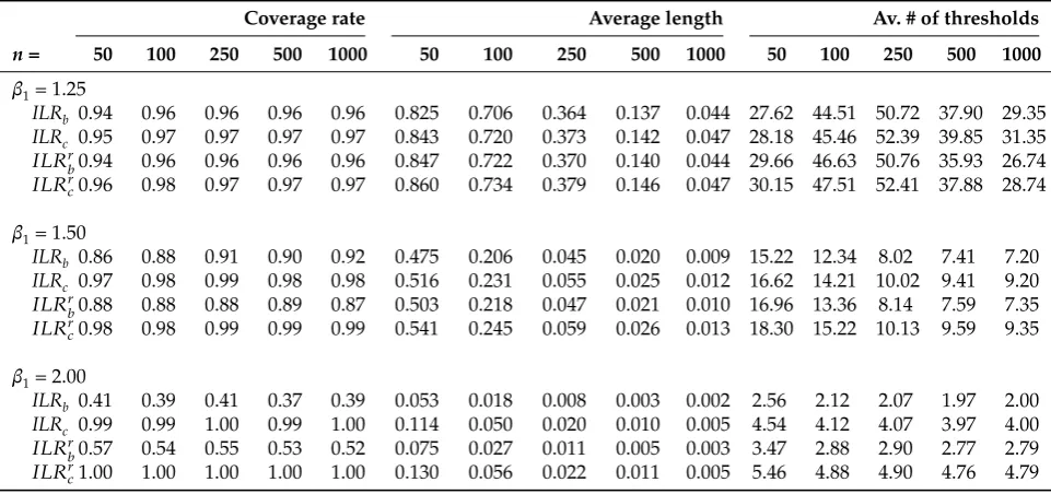
The results are reported in Table 1. The benchmark and conservative approaches using the standard grid-search areILR_bandILR_c, respectively. Those using the refined grid-search are𝐼𝐿𝑅𝑟_𝑏and𝐼𝐿𝑅𝑟𝑐, respectively. In all

cases, the refined grid-search approach generates confidence intervals with slightly higher coverage rates rel-ative to the standard grid-search approach, but the increase is only marginal. Therefore, our discussion below focuses on the distinction between the benchmark,ILRband conservativeILRc approaches, since the

perfor-mances of𝐼𝐿𝑅𝑟_𝑏and𝐼𝐿𝑅𝑟𝑐are similar to those, respectively.

When the threshold effect is small (β₁= 1.25), all approaches slightly overcover for most sample sizes, with

the exception of the ILRb approach which slightly undercovers forn = 50. As the threshold effect becomes

larger, theILRb approach produces coverage rates far below the nominal level. For example, whenβ1 = 2.00

the coverage rates of theILRbapproach range from 0.37 to 0.41 while, consistent with being conservative, the ILRcapproach always produces coverage rates greater than the nominal level, e.g. 0.99 to 1.00. Intuitively, the

identification of the threshold parameter is very precise as the threshold effect increases. Hence, the confidence intervals become very narrow and include very few points. This relatively small number of average threshold points results in a poor approximation to the profile likelihood for the threshold parameterγ. Our

interpreta-tion of this undercoverage for theILR_bapproach is supported by the average threshold points across Monte Carlo simulations included in the CIs: ranging from 7.2 to 15.2 forβ₁ = 1.5 and from 1.97 to 2.56 forβ₁= 2.0

depending on the sample size. Note that the average number of threshold points ranges from 27.6 to 50.7 when the threshold effect is small (β₁= 1.25) so that this large number of the threshold points help approximate the

profile likelihood. Meanwhile, the conservative approach can achieve significantly more accurate coverage rates at the cost of a trivial increase in the normalized average length of the CIs. This increase ranges from 0.3 to 6.1 percentage points.

Overall, the results of this Monte Carlo experiment suggest that the conservative approach can achieve more accurate coverage rates with a relatively marginal increase in the average length in comparison to the benchmark approach.

4.2 Monte Carlo experiment 2

In the second experiment, we generate data according to the following self-exciting TAR (SETAR) model:

𝑦𝑖=

⎧ { ⎨ { ⎩

𝛼0+ ∑

𝑝

𝑗=1𝛼𝑗𝑦𝑖−𝑗+ 𝑒𝑖, if𝑦𝑖−𝑑≤ 𝛾

𝛽0+ ∑

𝑝

𝑗=1𝛽𝑗𝑦𝑖−𝑗+ 𝑒𝑖, if𝑦𝑖−𝑑> 𝛾

(15)

To reduce the computational burden, we focus on the simplest case wherep=d= 1 and setα₀= 0,α₁= 0.3,β₀=

0.9,β₁= 0.6 andγ₀= 0. Because the DGP follows a SETAR model, it is not easy to measure the magnitude of the

threshold effect. Thus, we vary the error variance according toe_i∼i.i.d. N(0,σ2) fori= 1,…,nand setσ= 0.3, 0.5,

Aut

omatic

all

yg

ener

at

ed

rough

PDF

by

Pr

oo

fCheck

fr

om

Ri

ver

Valle

yT

ec

hnologies

Lt

d

effect. The DGP with a unit error variance was studied by Enders, Falk, and Siklos (2007), but we consider the various variance sizes to examine the impact of the magnitude of the threshold effect on the performance of the CIs. The sample size isn= 236, which is the same as in Enders, Falk, and Siklos (2007) .

Table 2 presents empirical coverage rates, average lengths and average number of threshold observations across different variance sizes. The results show that the benchmark approach,ILR_b, performs poorly when the threshold effect is large (i.e.σ= 0.3, 0.5) in the sense that the coverage rates are 0.41 and 0.84, which are far below

the nominal level. The refined grid-search procedure helps by accounting for non-observable threshold values, but the improvement is only marginal, resulting in the coverage rates of 0.55 and 0.84, respectively. Meanwhile, the conservative approach, ILRc, again consistent with being conservative, produces coverage rates that are

higher than the nominal level, overcovering the true threshold parameter, from 0.97 to 0.99 at the trivial cost of marginally longer confidence intervals. Note that the normalized lengths of the CIs based on theILRcapproach

are about 1.2 to 1.5 percentage points longer than those for theILRbapproach.

We find the poor performance of the benchmark approach occurs because the few threshold variable obser-vations included in the CIs produce a poor approximation to the profile likelihood, as argued in the previous section. The average number of the threshold observations in the CIs is 36 when the threshold effect is small (σ= 1). However, that number falls significantly (about 2 to 6 observations) when the threshold effect becomes

large (σ= 0.3, 0.5).

5 A counterfactual experiment

The coverage rates are determined by the frequency of Monte Carlo simulations for which the likelihood-ratio test is not rejected at the true threshold parameter value. In the previous sections, we argue that the true thresh-old value is likely to exist either in (q(l−1),q(l)) or in (q(u),q(u+1)) when the threshold effect is large, given the poor

approximation to the profile likelihood. Any threshold value either in (q(l−1),q(l)) or in (q(u),q(u+1)) leads to

reject-ing the test and this results in the poor performance of the CIs. Based on this argument, we have proposed the use of a conservative approach by extending the benchmark confidence interval to include all threshold values in [q(l−1),q(u+1)].

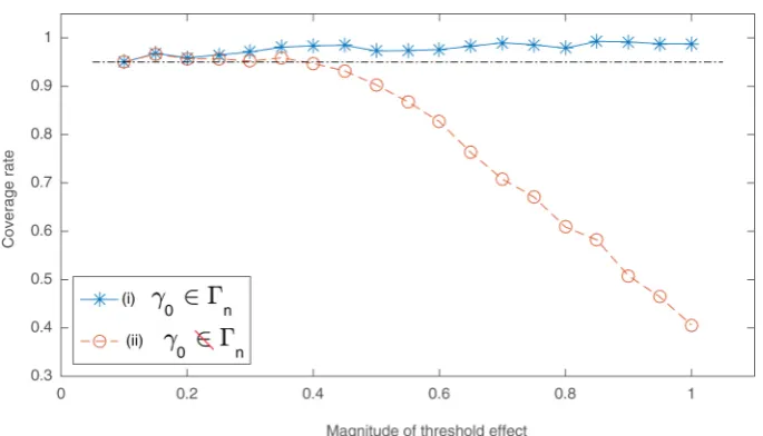
To examine whether our argument is valid, we conduct a counterfactual experiment. We repeat the first Monte Carlo experiment withn= 250 andβ₁= 1.10, 1.15,…, 2.00, but consider two different cases: (i) the true

threshold parameter𝛾₀∈ {𝑞𝑖}𝑛𝑖=1or (ii)𝛾0∉ {𝑞𝑖}𝑛𝑖=1. Thus, in case (i), we force the true threshold value to become observable when generating the threshold variable in the simulation. This setting is a counterfactual experiment because the true threshold value would be included in the data set of the threshold variable with probability 0 if the threshold variable were assumed to follow a continuous distribution as studied in the literature. In this case, the true threshold value must be equal to one of threshold variable observations.8_{Therefore, we can}

conduct the likelihood-ratio test at the true threshold value against the threshold estimate in each simulation without using the step function approximation:

𝐿𝑅𝑛(𝛾0) = 𝑛

𝑆𝑛(𝛾0) − 𝑆𝑛( ̂𝛾)

𝑆𝑛( ̂𝛾)

(16)

where𝛾₀∈ {𝑞𝑖}𝑛𝑖=1. Note that the threshold estimate is not necessarily equal to the true threshold value because the threshold estimate is determined by the threshold value which minimizes the SSR.

If our argument is correct, the simulation setting in case (i) would result in a rejection frequency of 5% or less at the true threshold value. Hence, the coverage rates would be equal to or greater than 95%.9 _{Case (ii)}

is the same as the Monte Carlo experiment setting in Section 4.1. We construct confidence intervals using the benchmark approach.

Aut

omatic

all

yg

ener

at

ed

rough

PDF

by

Pr

oo

fCheck

fr

om

Ri

ver

Valle

yT

ec

hnologies

Lt

d

6 Application: thresholds for US industrial production growth at a disaggregated

level

In this section, we compare the benchmark and conservative approaches to constructing confidence intervals for the threshold parameter for US industrial production growth at a disaggregated level. We use a SETAR model to examine asymmetric dynamics related to the business cycle. Our data set consists of 74 manufacturing industries that are closely related to the four-digit level of disaggregation in the North American Industry Classification System (NAICS). The data are for the sample period of 1972:Q1 to 2011:Q4 and were obtained from the Board of Governors of the Federal Reserve System.10_{Quarterly growth rates are calculated as 100 times}

the first differences of the natural logarithm of the level data.

Potter (1995) estimates a threshold model of US real GNP under the assumption that the threshold is known and equal to zero. Instead of using the assumed threshold value of zero, we estimate the threshold parameter and construct its confidence interval. In doing so, we examine if: (i) the threshold confidence intervals include zero across different industries; and, (ii) the two approaches (ILRbandILRc) make the same inference about the

threshold parameter based on the confidence intervals.

We first test for linearity for each industry and, if linearity is rejected, we then estimate the SETAR model and construct confidence intervals for the threshold parameter using the following model for each industryi

𝑦𝑖,𝑡 =

⎧ { ⎨ { ⎩

𝛼𝑖,0+ ∑

𝑝

𝑗=1𝛼𝑖,𝑗𝑦𝑖,𝑡−𝑗+ 𝑒𝑖,𝑡, if𝑦𝑖,𝑡−𝑑≤ 𝛾𝑖

𝛽𝑖,0+ ∑

𝑝

𝑗=1𝛽𝑖,𝑗𝑦𝑖,𝑡−𝑗+ 𝑒𝑖,𝑡, if𝑦𝑖,𝑡−𝑑> 𝛾𝑖

(17)

wherey_i,tis the quarterly growth for the industryi.

We employ Hansen’s (1996) heteroskedasticity-consistent Lagrange multiplier test for a threshold effect

in linear regression and calculate p-values using 1,000 bootstrap replications. Hansen (1996) shows that this bootstrap procedure produces asymptotically correct p-values. Constructing the confidence intervals takes into account the heteroskedasticity using a quadratic regression to estimate a nuisance parameter on which the asymptotic distribution ofLRn(γ) is dependent. See Hansen (2000) for more details.

We estimate the SETAR model withp=d= 1 in (17) and find that the null hypothesis of linearity is rejected for 12 industries at the 10% level, with two of these industries–Pharmaceutical and Medicine (NAICS 3254)

and Office and Other Furniture (NAICS 3372,9)–having a discrepancy in terms of the coverage of zero across

the two different approaches using 90% confidence intervals.11

Table 3 presents the summary of the linearity test results with p-values and the confidence intervals for the 12 industries.12_{The conservative approach includes zero in the threshold confidence intervals for 9}

indus-tries among 12 indusindus-tries for which the linearity test is rejected, while the benchmark approach does so for 7 industries only. Regarding the two industries in which the discrepancy in the coverage of zero in the confi-dence intervals is observed, the two approachesILR_bandILR_cproduce the confidence intervals of (0.064, 0.964) and (−0.016, 0.975), respectively for Pharmaceutical and Medicine industry and (−2.512,−0.002) and (−2.570,

0.136), respectively for Office and Other Furniture industry.

We note that this discrepancy is not direct evidence of superiority of the conservative approach (ILRc) we

propose the use of in this paper. It could be that the true threshold is not actually zero for any industry, as it appears not to be for at least three industries. However, our results show that the two different approaches can make empirically meaningful differences in an actual application. Moreover, because the Monte Carlo analysis suggests the conservative approach is more reliable in finite samples, the exclusion of zero in three cases is more credible than the exclusion of zero in the two additional cases for the benchmark approach.

7 Concluding remarks

Using Monte Carlo simulations, we have shown that asymptotically-valid likelihood-ratio-based confidence intervals may perform poorly, even for large samples, when the threshold effect is particularly large. The cov-erage rates of the benchmark confidence interval derived in Hansen (2000) are substantially below nominal levels. We have proposed a conservative modification to Hansen’s benchmark approach and this modification

Aut

omatic

all

yg

ener

at

ed

rough

PDF

by

Pr

oo

fCheck

fr

om

Ri

ver

Valle

yT

ec

hnologies

Lt

d

Acknowledgement

We thank two anonymous referees, Sunoong Hwang, Adrian Pagan, and Christopher Parmeter for useful com-ments. All errors are our own.

Appendix: Tables

Table 1:Monte Carlo experiment 1.

Coverage rate Average length Av. # of thresholds

n= 50 100 250 500 1000 50 100 250 500 1000 50 100 250 500 1000

β₁= 1.25

 ILR_b 0.94 0.96 0.96 0.96 0.96 0.825 0.706 0.364 0.137 0.044 27.62 44.51 50.72 37.90 29.35  ILR_c 0.95 0.97 0.97 0.97 0.97 0.843 0.720 0.373 0.142 0.047 28.18 45.46 52.39 39.85 31.35  𝐼𝐿𝑅𝑟

𝑏0.94 0.96 0.96 0.96 0.96 0.847 0.722 0.370 0.140 0.044 29.66 46.63 50.76 35.93 26.74

 𝐼𝐿𝑅𝑟

𝑐0.96 0.98 0.97 0.97 0.97 0.860 0.734 0.379 0.146 0.047 30.15 47.51 52.41 37.88 28.74

β₁= 1.50

 ILRb 0.86 0.88 0.91 0.90 0.92 0.475 0.206 0.045 0.020 0.009 15.22 12.34 8.02 7.41 7.20

 ILR_c 0.97 0.98 0.99 0.98 0.98 0.516 0.231 0.055 0.025 0.012 16.62 14.21 10.02 9.41 9.20  𝐼𝐿𝑅𝑟_𝑏0.88 0.88 0.88 0.89 0.87 0.503 0.218 0.047 0.021 0.010 16.96 13.36 8.14 7.59 7.35  𝐼𝐿𝑅𝑟

𝑐0.98 0.98 0.99 0.99 0.99 0.541 0.245 0.059 0.026 0.013 18.30 15.22 10.13 9.59 9.35

β₁= 2.00

 ILR_b 0.41 0.39 0.41 0.37 0.39 0.053 0.018 0.008 0.003 0.002 2.56 2.12 2.07 1.97 2.00  ILRc 0.99 0.99 1.00 0.99 1.00 0.114 0.050 0.020 0.010 0.005 4.54 4.12 4.07 3.97 4.00

 𝐼𝐿𝑅𝑟

𝑏0.57 0.54 0.55 0.53 0.52 0.075 0.027 0.011 0.005 0.003 3.47 2.88 2.90 2.77 2.79

 𝐼𝐿𝑅𝑟𝑐1.00 1.00 1.00 1.00 1.00 0.130 0.056 0.022 0.011 0.005 5.46 4.88 4.90 4.76 4.79

For the first experiment, we consider a threshold model with the following DGP:

𝑦𝑖=

⎧ { ⎨ { ⎩

1+ 𝑥𝑖+ 𝑒𝑖, if𝑞𝑖≤2 1+ 𝛽1𝑥𝑖+ 𝑒𝑖, if𝑞𝑖>2

wherexi=qi∼N(2, 1) andei∼i.i.d.N(0, 1) fori= 1,…,n. The average lengths are normalized by the length of the bounded parameter

spaceΓ= [𝛾, 𝛾]for each sample size, while the average number of threshold observations is expressed as a percentage of the sample size.

Table 2:Monte Carlo experiment 2.

Coverage rate Average length Av. # of thresholds

σ= 1.0 0.5 0.3 1.0 0.5 0.3 1.0 0.5 0.3

ILR_b 0.95 0.84 0.41 0.284 0.038 0.008 36.00 5.71 2.04

ILRc 0.97 0.99 0.99 0.294 0.050 0.023 37.78 7.71 4.04

𝐼𝐿𝑅𝑟_𝑏 0.95 0.84 0.55 0.288 0.040 0.012 37.13 6.93 2.99

𝐼𝐿𝑅𝑟

𝑐 0.98 0.99 1.00 0.299 0.052 0.024 38.90 8.93 4.99

We consider a SETAR model and setσ= 1.0, 0.5, 0.3 for the error variance. The DGP is given by

𝑦𝑖=

⎧ { ⎨ { ⎩

0.9+0.6𝑦𝑖−1+ 𝑒𝑖, if𝑦𝑖−1≤0 0.0+0.3𝑦𝑖−1+ 𝑒𝑖, if𝑦𝑖−1>0

whereei∼i.i.d.N(0,σ2) fori= 1,…,nandn= 236. The average lengths are normalized by the length of the bounded parameter space Γ= [𝛾, 𝛾]for each sample size, while the average number of threshold observations is expressed as a percentage of the sample size.

Aut

omatic

all

yg

ener

at

ed

rough

PDF

by

Pr

oo

fCheck

fr

om

Ri

ver

Valle

yT

ec

hnologies

Lt

d

NAICS Industry description Linearity test Threshold 90% confidence interval (p-Value) Benchmark Conservative 3114 Fruit and vegetable preserving and

specialty food 0.066 (−2.455, 2.979) (−2.491, 3.114)

3254 Pharmaceutical and medicine 0.030 (0.064, 0.964) (−0.016, 0.975) 3256 Soap, cleaning compound, and toilet

preparation 0.070 (0.787, 3.299) (0.750, 3.304)

3314 Nonferrous metal (except aluminum)

production and processing 0.084 (−5.070, 3.936) (−5.070, 3.936) 3329 Other fabricated metal product 0.005 (−0.329, −0.329) (−0.349, −0.306) 3331 Agriculture, construction, and mining

machinery 0.029 (−4.468, 4.832) (−4.491, 4.897)

3332 Industrial machinery 0.044 (−3.457, 4.179) (−3.877, 4.279) 3336 Engine, turbine, and power

transmission equipment 0.067 (−3.851, 4.369) (−3.851, 4.369) 3342 Communications equipment 0.032 (−1.547, −0.489) (−1.620, −0.456) 3364 Aerospace product and parts 0.001 (−2.425, 1.536) (−2.507, 1.560) 3369 Other transportation equipment 0.000 (−4.058, 6.698) (−4.058, 6.698) 3372,9 Office and other furniture 0.039 (−2.512, −0.002) (−2.570, 0.136) We consider a SETAR model:

𝑦_𝑖,𝑡=⎧{_⎨ { ⎩

𝛼_𝑖,0+ 𝛼𝑖,1𝑦𝑖,𝑡−1+ 𝑒𝑖,𝑡, if𝑦𝑖,𝑡−1≤ 𝛾𝑖

𝛽_𝑖,0+ 𝛽𝑖,1𝑦𝑖,𝑡−1+ 𝑒𝑖,𝑡, if𝑦𝑖,𝑡−1> 𝛾𝑖

whereyi,tis the quarterly growth for the industryi. The 90% confidence intervals for the threshold parameterγithat do not include zero

are in bold.

Appendix: Figures

Figure 1:Illustrated example of log-likelihood ratio profile for the threshold parameter.

Note: A hypothetical LR profile is depicted. Given a finite number of observations of the threshold variable, the like-lihood ratio is evaluated discretely. Thus, for allqi∈[q(j),q(j+ 1)), there is the same likelihood ratio valueLRn(qi) =

LRn(q(j)), denoted by a dashed line. The left endpoint of the intervalq(j) is denoted by a solid point and the right endpoint

Aut

omatic

all

yg

ener

at

ed

rough

PDF

by

Pr

oo

fCheck

fr

om

Ri

ver

Valle

yT

ec

hnologies

Lt

d

Figure 2:Counterfactual experiment. Note: The true threshold parameter isγ₀and the magnitude of the threshold effect

is measured byδ=β₁−α₁.

Notes

1 For a comprehensive review of threshold applications in economics, see Hansen (2011), Tong (2011), and Gonzalo and Pitarakis (2013) . 2 Although we only consider two regimes, we note that Hansen (1999) argues that results in Hansen (2000) will hold for multiple thresh-olds. Also, Eo and Morley (2015) consider a related approach in the context of structural breaks and find that multiple breaks do not make a difference in comparison to a single break case.

3 Assumptions made in this paper are equivalent to those in Hansen (2000) and we omit these for brevity.

4 Similarly, it is possible that there are some threshold parameter values𝛾 ∈ (𝑞(𝑙 −̀ 1), 𝑞(𝑙))such that𝐿𝑅𝑛( ̀𝛾) ≤ 𝐶𝑅1−𝛼where𝑞(𝑙 −1) = max{𝑞𝑖∶ 𝐿𝑅𝑛(𝑞𝑖) > 𝐶𝑉1−𝛼, 𝑞𝑖< 𝑞(𝑙), 𝑞𝑖∈Γ𝑛}.

5 Too few observations in the confidence intervals mean that there is not enough information to approximate the LR profile and to correctly make inferences about the true threshold parameter. We confirm this conjecture in our Monte Carlo simulations.

6 As is standard in the literature, we trim the first and last 15% (i.e.ϵ= 0.15) of the threshold observations for both grid-search procedures

in our Monte Carlo simulations, counterfactual experiment, and application. We have confirmed that the results are robust to alternative trimming values of 5% or 20%. Results are available from the authors upon request.

7 We have confirmed that the Monte Carlo results are robust to alternative confidence levels of 90% and 80% in the sense that the methods that undercover relative to the nominal level continue to do so, while the conservative approach, consistent with being conservative, always overcovers, but not by as much as the other methods undercover. Results are available from the authors upon request.

8 In the context of structural breaks, the true structural break date, which is equivalent to the true threshold value in threshold models, is always one of the observed dates in the sample, if it exists and is within the trimmed set. This can explain why Eo and Morley (2015) find that the likelihood-ratio-based approach to constructing confidence intervals for structural breaks always performs well, regardless of the magnitude of structural break effects.

9 Note that the likelihood-ratio test is conservative when the threshold effect is large (see Theorem 3 in Hansen 2000).

10 Chang and Hwang (2015) use the same data set to identify cyclical turning points and their comovement and asymmetry. For compa-rability, we consider the same sample period as in their paper. See Chang and Hwang (2015) for more details on the data.

11 We confirm that settingp=d= 1 is the preferred specification based on the Schwarz information criterion for these two industries when allowingp= 1,…, 5 andd= 1,…, 5.

12 We report the results for the industries for which the linearity test is rejected to save space.

References

Balke, Nathan S. 2000.“Credit and Economic Activity: Credit Regimes and Nonlinear Propagation of Shocks.”The Review of Economics and Statistics82: 344–349.

Chan, Kan S. 1993.“Consistency and Limiting Distribution of the Least Squares Estimator of a Threshold Autoregressive Model.”Annals of Statistics21: 520–533.

Chan, Kan S., and Ruey S. Tsay. 1998.“Limiting Properties of the Least Squares Estimator of a Continuous Threshold Autorregressive Model.” Biometrika45: 413–426.

Chang, Yongsung, and Sunoong Hwang. 2015.“Asymmetric Phase Shifts in US Industrial Production Cycles.”Review of Economics and Statistics 97 (1): 116–133.

Enders, Walter, Barry Falk, and Pierre Siklos. 2007.“A Threshold Model of U.S. Real GDP and the Problem of Constructing Confidence Inter-vals in TAR Models.”Studies in Nonlinear Dynamics and Econometrics11 (3): Article 4.

Aut

omatic

all

yg

ener

at

ed

rough

PDF

by

Pr

oo

fCheck

fr

om

Ri

ver

Valle

yT

ec

hnologies

Lt

d

Gonzalo, Jesús, and Jean-Yves Pitarakis. 2013.“Estimation and Inference in Threshold Type Regime Switching Models.”InHandbook of Re-search Methods and Applications in Empirical Macroeconomics, edited by Nigar Hashimzade and Michael A. Thornton, 189–204. Cheltenham: Edward Elgar Publishing Limited.

Hansen, Bruce E. 1996.“Inference When a Nuisance Parameter is Not Identified Under the Null Hypothesis.”Econometrica64: 413–430. Hansen, Bruce E. 1997.“Inference in TAR Models.”Studies in Nonlinear Dynamics and Econometrics2 (1): 1–14.

Hansen, Bruce E. 1999.“Testing for Linearity.”Journal of Economic Surveys 13: 551–576. Hansen, Bruce E. 2000.“Sample Splitting and Threshold Estimation.”Econometrica68: 575–603. Hansen, Bruce E. 2011.“Threshold Autoregression in Economics.”Statistics and Its Interface4: 123–127.

Koop, Gary, and Simon Potter. 2004.“Dynamic Asymmetries in U.S. Unemployment.”Journal of Business and Economic Statistics17 (3): 298–312. Potter, Simon. 1995.“A Nonlinear Approach to U.S. GNP.”Journal of Applied Econometrics10: 109–25.

Tong, Howell. 2011.“Threshold Models in Time Series Analysis–30 years on.”Statistics and Its Interface4: 107–136.

Supplemental Material: The online version of this article offers supplementary material (DOI: