NEW PROPERTIES OF THE TWO-LOCUS PARTIAL SELFING MODEL WITH SELECTION

NEW

PROPERTIES

OF THE

TWO-LOCUS

PARTIAL

SELFING

MODEL WITH

SELECTION1

L. R. HOLDEN2

Division of Biological Sciences, University of Kansas, Lawrence, Kansas 66045

Manuscript received February 9, 1978

Revised copy received March 9,1979

ABSTRACT

Analytic solutions are obtained for the equilibria of a simple two-locus, heterotic selection model with mixed selfing and random outcrossing. T W O

general phenomena are possible, depending upon the viabilities and the degree of selfing: ( I ) Negative disequizibrium potential, under which only gametic disequilibrium is possible; and (2) positive disequilibrium potential, which can result in permanent gametic disequilibrium provided that linkage is sufficiently tight. Under random mating (s = O), these two situations correspond to nega- tive and positive additive epistasis, respectively. With partial self-fertilization, however, this is no longer true, and a more appropriate measure of gametc dis- equilibrium potential, A (s)

,

is introduced. A numerically aided examination of the model results in the discovery of two new properties of partial selfing with selection: (1) With negative disequilibrium potential (A(s)

<

0), the equi- librium mean fitness increases with increasing recombination. With positive disequilibrium potential (A(s)

>

0), the opposite is true. (2) Gametic disequi- librium can increase or decrease as the degree of selfing is increased. There- fore, it is apparent that partial selfing and linkage are not analogous as regards the maintenance of disequilibrium.

M U C H attention has recently been given to the effects

of selection on the eqwlibrium structure of multilocus systems. This increased interest is due,

in no small part, to the discovery of large amounts of genetic diversity in natural populations and the inability of single-locus theory to provide a satisfactory ex- planation for its maintenance. One commonly proposed cause for such diversity is some form of heterotic selection. If each locus is subjected to overdominant se- lection “independently” of the rest of the genome, then the population must con- tend with the many lesser fit segregational genotypes that result i n a very low mean relative fitness. Whether or not such a segregational “load” on

the

popu- lation is actually evolutionarily harmful, it is still true that the population will

be less fit in the short run than an equivalent asexual population. If, however, some alleles at different loci tend to “work better together” than others, then these tend to be forced into close association by selection. Such association of alleles at different loci,

if

present, would allow heterotic selection to proceed without the production of the numerous segregational genotypes.

l This research was supported in part by National Science Foundation Grant BM573-01305 to PEULXP W. HEDRICK

*

Present address: Research Department, Monsanto Agricultural Products Co., 800 North Lindbergh Boulevard, St.

and by a University of Kansas Dissertation Fellowship.

Louis, Missouri 63166.

218 L. R. HOLDEN

The search for such interlocus associations or “gametic disequilibrium” in nature, often considered p r i m a facie evidence for such nebulous phenomena as “coadaptation” or “epistasis,” has also stimulated theoretical developments (see discussion in HEDRICK,

JAIN

and

HOLDEN

1978). Advances in multilocus theory to date have been very encouraging. KARLIN (1975) reviews and extends the results of the two-allele, two-locus, random-mating model, presenting several general principles for multilocus selection as well. Recent advances in multiple- allele, two-locus theory have been made by FELDMAN et al. (1975) and CHRIS- TIANSEN and FELDMAN (1975) and in three-locus theory by FELDMAN, FRANK- LIN and THOMSON (1974), STROBECK (1973, 1976) and KARLIN and LIEBER- MAN (1976). I n addition, multilocus computer simulation studies (FRANKLIN and LEWONTIN 1970; YAMAZAKI 1977;

WILLS

and MILLER 1977; CLEGG 1978) have provided considerable insight into the maintenance of polymorphisms and interlocus associations with large numbers of loci. However, it is clear that with more complex fitness models the relationship between linkage and disequilib- rium, even with random mating, is quite complex (e.g., EWENS 1969).

I n almost all selection studies, however, random mating is assumed; the nota- ble exceptions being the complete selfing model ( SHIKATA 1963) and the detailed numerical studies of heterotic and optimizing selection in partial selfing popula- tions (JAIN and ALLARD 1966;

JAIN

1968, 1969). Although considerations of models with random mating certainly need no justification, inbreeding is also important. In fact, a regular system of inbreeding, partial self-fertilization, is common in plants. It is interesting that some of the most notable natural exam- ples of interlocus association among electrophoretic loci occur in barley ( WEIR,

ALLARD and KOHLER 1972) and in wild oats (CLEGG, ALLARD and KAHLER 1972; ALLARD et al. 1972), both predominantly selfing species. I n all of these cases, the authors were forced to advance explanations without the aid of much multilocus inbreeding theory, although more has since been done (e.g.,

WEIR

and COCKER- HAM 1973). The only selection “theory” available consisted of the general belief that increased inbreeding is analogous to tighter linkage in its effect upon the pro- duction and maintenance of gametic disequilibrium (see ALLARD, JAIN and

WORKMAN

1968, for example). In this paper,

I

attempt to advance the theory of multilocus selection with inbreeding by presenting an analytic solution to a simple two-allele, two-locus, partial selfing, heterotic selection model. Although concerned with a specific fitness model, the results indicate that the relationships among selection, selfing and recombination are much more complex than commonly assumed.

DESCRIPTION O F THE MODEL

TWO-LOCUS SELECTION WITH INBREEDING 219

component gamete types

( i

5

i and

i,j

= 1 , 2 , 3 , or 4. Similarly, the relative via- bility of each genotype

(ij)

will be denoted by wi j.

Generations will be assumed to be discrete and nonoverlapping and viability selection assumed to operate on only the premating diploid organisms. The fre- quency of genotype

(i>j)

after selection but before mating, is then given by:

where

is the mean relative fitness of the population.

Inbreeding is imposed on the population by assuming that selfing occurs with frequency s and random outcrossing with frequency l-s. The system

of

equations relating the genotypic frequencies after mating, gzj, with those before mating, g’,j are:

gl

=s{g’ll

+

% ( g 1 2

+

g’13

+

c2g‘23

+

(1-c)2g‘14)}

+

(l-s) (2’1)’ y*2 = d g ’ 2 2

+

%

(g’iz

+

g z 4 f C2g’i4

+

(1-C>2g)23)} f (1-S) ( 9 2 ) ’

z 3 3 = s{g33

+

% ( & I S

+

g’34

+

c2g‘14

+

(1-c>2gz3)}

+

(1-S) (2’3)’

-

g41 = S(g’44

+

%

(g21f g ’ 3 4 f c2g’23

+

(1-c)2g14)} f (l-s) (x’4)2

zfj

= 1/2s{g’lj

+

c(1-c) ( g ‘ i a +g)23)}

+

(l-s)gx’iZ’j 7 (2)

for

(i,j)

= (I$), (1,3), (2,4), (3,4) z14=l/zs{(l-c)2g’14fC2g’23}

+

(1-s)22‘12’4

2 2 3 = l / S { (1-C)2g‘z3 f CZg’14}

+

(1-.9)22’25’3

,

where

x’i g‘ii

+

%

2 g’ii’ f

%

g k i - S i

i/z

c(g‘14

-

g’14

-

g’23)

,

I < % k<i

6, = 6, = 1, 6, =

s3

= -1

,

and c denotes the recombination fraction between locus A and locus

B

(0 2

c 2

s ) .

Combining ( 1 ) and (2) results in a system of equations relating the

genotypic frequencies in two successive generations. By setting

gj

=gij, the sys- tem (1,2) can be solved to yield the frequencies at equilibrium. For 0

<

s

<

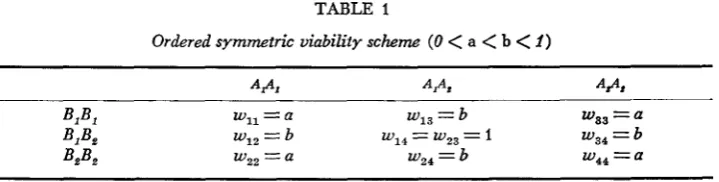
1, no general analytic solution has yet been obtained, although numerical solutions are possible ( JAIN and ALLARD 1966).

Let us consider, however, a model where all the double homozygotes have rela- tive viability a, the single heterozygotes have viability b and both types of double heterozygotes have a relative viability of 1 (see Table 1 )

,

where 0

<

a

<

b

<

1 . This is a special case of the fitness pattern first considered by

LEWONTIN

and KOJIMA (19SO). If it is assumed that pl = q1 =

%,

it can easily be verified that at equilibrium:

gll = g 4 4 7 g 2 2 =r g33, g12 = g13 = g24 = g34

.

220 L. R. HOLDEN TABLE 1

Ordered symmetric viability scheme ( 0

<

a

<

b

<

I )

A P , A,** A#*

Wll = a w13 = b ws3 = a

BIB, wI2 = b W14 = wz3 = I w34 = b w~~ = a

4%

wz2 = a wz4 = b

BIB,

be unequal. I n order to make such contributions more apparent,

I

introduce the

gametic imbalance parameter,

Y ,

defined as:

Y

= (z,

+

2 4 )

-

( 5 2

+

x3)

= gll

+

g14

+

g44

-

g 2 2

-

g 2 3

-

g33

y h m

+

Y h e t 7

(4)

where

Y h o m = (g11+ g44)

-

(gzz

+

g33)

Y h e t = gl4

-

g 2 3 *

Thus Y h o m and Y h e t represent the gametic imbalance in homozygotes and h

double heterozygotes, respectively. This gametic imbalance parameter is related to the traditional measure of disequilibrium,

D

=

5 1 2 4

-

22x3, by

4D

=

Y

-

(PI-%)

(ai--%>

*

Strictly speaking, Y does not measure the deviation from between-locus inde- pendence of the frequencies of alleles (gamete disequilibrium), but rather the degree to which the complementary gamete pair { (A,B,), (A,B,)} predominates over the pair { ( A I B P ) , ( A , B , ) } . However, at polymorphic equilibria with pl

=

q l =

%:

Y = Y h m

+

Y h e t =

4D

,

and thus Y also measures gametic disequilibrium.

By defining

H

= g14f g 2 3 and h = glz =g13 = gZ4 = g34, we can now express all ten equilibrium genotypic frequencies in terms of the four parameters

H ,

h,

r h o , and Y h e t :

g14 =z

%

( H

+

Y h e t ) , g 2 3 =

1/2

( H

-

Y h e t ) ,

gii = g44=

%

(1

-

h

-

4.H Y h o m ) ,

(6)

gzz = g 3 3

%

(1

-

h

-

4H

-

Y h o m ) 7

gl2 = g13 gZ4 = g34 = *

TWO-LOCUS SELECTIOh- WITH INBREEDING

S

h =- ( I - ) (1-T2)

+

-

{bh

+

c ( 1 - c ) H )

8

2w

H = - - ( l + T Z ) (1.-s)

+ - { % -

S

4 W ~ ( l - c ) }

H

where

and the mean relative fitness becomes

W

= a

+

( l - a ) H

+

4 ( b - a ) h

.

(8)

This reduced system can then be solved for the two possible classes ofjequi- libria: ( 1 ) a gametic equilibrium ( Y = 0), or “central,” solution; and ( 2 ) a

‘‘noncentral” class of equilibria for which Y # 0.

The noncentral equilibria

Let us first consider Y # 0 at equilibrium. It is shown in the APPENDIX that with the restrictions on the viabilities (Table 1 ) and on s and c, Yhet and Yhom

are of the same sign at equilibrium. I n addition,

Yf

0 implies that

both

Yhet # 0

and Yhoea # 0. Using this fact, we can solve for W in the equilibrium equations (7a) and (7b) to obtain:

(f+s)a (I-%) Yhet

2 + 2 Yhom

W =

and

By equating the right-hand sides of (9a) and (9b) weget:

which gives:

(1-2c)Yhet2

+

{ ( l + s > a - ( l - 2 ~ ) } ( Y h e t ) (Yhom)

-

(l-s)aYhom2= 0,

Yhet =

where

(1-2c)

-

( l + s ) a

Q = 2(1-2c)

Now since Q

<

R, the quantity

Q

’- R is negative. This would yield the incon-

222 L. R. HOLDERT

U = Q

+

R, the appropriate linear relationship between Yhom and Yhet at a non-

central equilibrium then becomes:

Substituting U = Yhet/Yhonf into (9a), we get

( l + s ) a + (1-2c)U

W=--

2 2

= ?4{(1-2~) + a ( l + s )

+

({(1-2c)+a(lS~)}'- 8 a s ( 1 - - 2 ~ ) ) ~ ~ } ,

c # i / ,

.

(13)

Assuming c = 1/2, the mean relative fitness found from (9a) is

w =

1/2(l+s)a

<

a

.

Since it is impossible for the mean fitness to be less than the viability of the least fit genotype. we must conclude that no stable gametic disequilibrium is possible with c =

s.

Thus. it has been shown that, at all noncentral equilibria, Yhet is directly pro- portional to Y7,01,f. Furthermore, the mean relative fitness of all these equilibria, if they exist, is the same and does not depend upon the viability of the single- locus heterozygotes, b.

Now from ( 7 ) above.

1 1

T =

w

(CLY71ont -I- (I-&) Yh,,} =

-

{ a f (I-2C)U)Yhont

W

Letting

1

B = - { a + (1-2c)u)

,

I W

then (7a) becomes

Solving (14) for YT,,,,,~~, we get

y 4 - H + - 1

hmn -

P2

'

where

4 ( W - s { i / Z -c(l-c)})

(1-s)

w

-~

+ =

TWO-LOCUS SELECTION WITH INBREEDING 223 In addition, since Y h e t = uYhom and

Y

,= Y h e t

+

Y h o w :

(15b)

V

Yhet = i.

-

( H + - 1) %, with same sign as Yhom ;

B

and, of course,

D

= %Y . There appear, therefore, to be two complementary noncentral equilibria: one with Y

>

0 and the other with

Y <

0.

Equation (7c) now becomes:

sbh + sc(l-c)H

2 w

h=- (1

-

(H+- I ) }

+w

8 or

where y and z are defined as:

z = c(1-c).

Using the definition of

+

above and letting p = 1 - s/2W,

Y f O

Finally, substituting (16) for h in the expression for mean relative fitness (8)

and solving for H :

(17) ( W-a) y

-

( 1-s) (b-a)

( 1 - a ) y - 2(b-a)p

H =

provided, of course that:

y # O and (1-a)~-2(b-a)p#O0.

Therefore, the two noncentral equilibria are completely specified by equa- tions ( 13)

,

( I 5)

,

( 16) and ( I 7). Both of these equilibria exist provided that:

and

H d

>

1, Y f O

(1-a)y - 2(b-a)p # 0.

I n addition, because all genotypic frequencies are nonnegative and sum to unity,

the implicit conditions:

O < H < I , O < h S ? & 0 _ < 4 h + H < 1 (18b)

224 L. R. HOLDEN The central equilibrium

Under the assumption that Y = 0 at equilibrium, equations (7a) and (7b) vanish. After some rearrangement, the remaining two equilibrium equations,

(7c) and (7d), become:

and

$& (1-s)W = (2W - sb) h -

SZH

% ( l - s ) W = { W - s ( l / - z ) } H ,

respectively, where z = c (1 - c ) as before. Since

W

= a

+

(1

-

a ) H

+

4( b

-

a ) h , equations (19) contain only the variables H and h.

I

have not been able to obtain explicit expressions for H and h from (19) and have resorted to numerical solutions. For example, solving (19) f o r

H

and h in terms of

W

yields:

(1-s)W 2{2W -S(l-22)}

H =

(1-S) W { ~ W - S ( I - ~ Z ) }

h =

4(2W-~b) {2W--~(I-22)}

’

for

W

# l / s b o r W # s (

l/

-

z )

.

Substituting these values into W-a = (l-a)H

+

4

(b--a) h, we get the relation:

.

(21) ( I-a) ( I -s)

w

2{2W--s( 1-22)}

(b-a) (1 -s> W(2W-s (1

-4~)

1

(2W-sb) {2W--s(l-22)}

+-

W-a

=

This cubic equation in

W

can then be solved numerically for the root in the interval:

max { X s b , s(X-2))

<

W

<

1

.

(22) I t is easily verified from (19) that some of the natural restrictions (18b) are violated for

W

outside this interval,

THE NATURE O F THE EQUILIBRIA

Review of the random mating case

Now that the equilibrium genotypic frequencies can be determined, it is neces- sary to specify to which equilibrium a population will eventually converge. Since the csual techniques of stability analysis (see KARLIN and FELDMAN 1970, for example) become too unwieldy when there is nonrandom mating, I have chosen a less rigorous but perhaps more heuristic approach. The well known stability properties for this model under random mating

(LEWONTIN

and KO-

TWO-LOCUS SELECTION WITH INBREEDING 225

Under random mating, the central equilibrium always exists and its mean viability is

W*

=

(1

+

a

+

2b), which is independent of c. The

two

non- central equilibria, when they exist, each have mean viability $ ( c ) =

i/z

(1

+

a )

-

c. The central equilibrium is unstable whenever the noncentral equilibria exist and stable (globally) when they do not. The noncentral equilibria are (locally) stable whenever they exist, which occurs only if:

d q c )

>

w*,

(23)

which is equivalent to the condition c

<

$4+ ( 1

+

a

-

2b).

define

In addition, the viability values can produce two types of phenomena. If we

A = $(o)

-

W * = ~(1+a--2b),

(24)

then, if A

<

0, selection and random mating, acting in concert, eventually elimi- nate any association of alleles between loci

(i.e., Y

= 0 ) . This will occur even if

there is complete linkage (c = 0)

,

provided all gametes are initially present.

If

A

>

0, however, then with complete linkage, selection and mating will

force two of the gametic types, either AIB, and A,B, or AIB, and AZB, to fixation. Thus

Y

would become either 1 or -1, respectively. Under such forces, only the action of recombination (c

>

0) can maintain all four gametic types i n the popu- lation and

I

Y ]

<

1. These are the two noncentral equilibria, and they exist for c

less than the critical value given above. For c greater than this value, recombina- tion is too strong to allow any maintenance of gametic disequilibrium.

TURNER

(1969) has termed the condition A

<

0 underepistasis and that of A

>

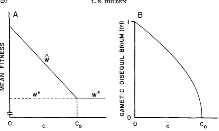
0 as over- epistasis. For reasons made clear later, I prefer the terms negative and positive disequilibrium potential for these two situations, respectively.

The general relationship between existence and stability of the equilbria and their mean viabilities are illustrated in Figure 1. Here, there is disequilibrium potential ( A

>

0) and the noncentral equilibria (

I

Y

I >

0) exist as long as c is less than the critical value denoted by co. For looser linkage, Figure l a shows that

6'(c) decreases as c increases. If ~ ( c ) =

W * ,

then c = co and the central equi- librium is stable for this and larger values of the recombination fraction. Figure 1 b also illustrates how the magnitude of gametic disequilibrium decreases from one to zero as the mean viability decreases from I@(O) to W * . If there were no (positive) disequilibrium potential, then the central equilibrium would always be stable and the mean viability equal to W* for all values of c .

Extensions to partial selfing

parameter of (24) generalizes to:

For any given value of s less than unity the gametic disequilibrium potential

(25 )

where I.i/(c,s) and W * ( c p ) are the mean relative viabilities at the noncentral and central equilibria, respectively. If the relation between A(s) and gametic

L. R. HOLDEN

0

A

\

\

I t

I

C

-

I -

>

-

Y

0

B

C

FIGURE 1.-(a) The typical relationship between recombination ( c ) and relative mean fitness for central ( W * ) and noncentral (I?) equilibria under random mating (s = 0) and positive disequilibrium potential (A

>

0). The solid line indicates a stable equilibrium.

(b) The corresponding decrease in the magnitude of gametic disequilibrium, IYl, with increasing recombination.

disequilibrium for s

>

0 is analogous to that for random mating, then we would predict that:

(i) For ~ ( s )

<

0, no gametic disequilibrium potential exists and only the central equilibrium (with Y = 0) is stable regardless of the recombination fraction.

(ii) For A ( s )

>

0, the noncentral equilibria exist and are stable for c less than than some critical value, co.

Examination of a large and representative number of €itness arrays, using com- puter simulation, failed to produce a single exception to (i) or (ii). Thus, we may safely infer that A ( s ) is an indicator of gametic disequilibrium potential for all s less than one.

A convenient means of determining the conditions under which

a

( s ) = 0 can be obtained by substituting W ( 0 , s ) for W* (0,s) in ( 2 1 ) . It is easily verified that this relation is satisfied if:

( l - a ) ( 2 % - s b ) = 2 ( b - a ) ( 2 W - s ) ,

-

-

where W = fi(0,s). Solving for b we get

-

W ( l + a ) -as

b = b =

2 w - i/z(l+a)

Y

N

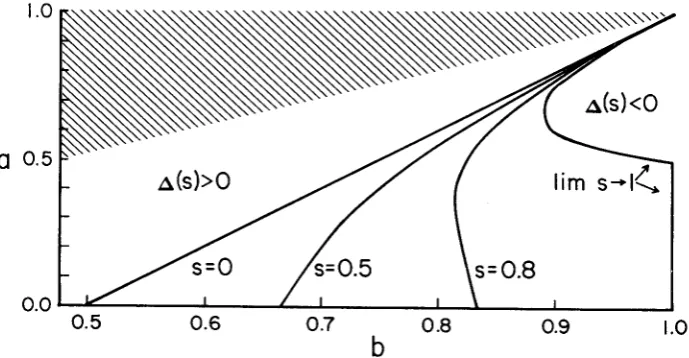
TWO-LOCUS SELECTION WITH INBREEDING 22 7 The relation ( 2 6 ) illustrates that disequilibrium potential occurs under a much wider range of conditions for partial selfing than for random mating. This

is shown in Figure 2, where b is plotted against a for various values of the selfing fraction. For all values of b to the left of a specific curve positive disequilibrium potential exists. For a 5

1/2,

disequilibrium potential is assured for all permissi- ble values of b provided s is increased sufficiently. However, for a

>

i/e,

lim

b

=

2a2/(3a

-

1 )

<

1, so that there do exist some values of b for which there is no (positive) disequilibrium potential possible for any degree of partial selfing.

For this model under random mating, the traditional additive (fitness) epista- sis parameter, E = 1

4-

a

-

2b, is directly proportional to A. Thus positive (over)

and negative (under) epistasis imply positive and negative disequilibrium poten- tial, respectively. With some deviation from random mating, E is no longer very

informative. For the viability pattern examined here at least, the more general A ( s ) is the appropriate parameter for determining the potential for gametic dis- equilibrium. I do not, however, wish to suggest that A ( s )

be

a new definition of epistasis on the fitness scale. It would seem to be more natural to separate the selective force tending to produce gametic disequilibrium (i.e., epistasis) from the disequilibrium potential resulting from the combined action of selection and the particular mating system.

The partial selfing extension of the condition for existence and stability of the noiicentral equilibria (23) is

-

U

8+ 1

fi(c,s)

>

w *

(c,s). ( 2 7 )

Again, in every case I have examined, ( 2 7 ) was found to delimit the conditions for stability of the noncentral equilibria. Figure 3 illustrates the general rela-

a

I

.o

0.5

0.0 I

.o

0.5

0.0

0.5

0.6 0.7 0.8 0.9 I I I

.o

.o

b

”

228 L. R. HOLDEN

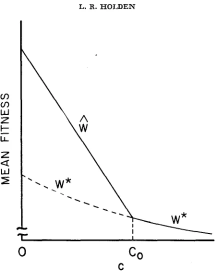
7- I

0

C O

C

FIGURE 3.-The typical relationship between equilibrium mean fitness and recombination for 0

<

s

<

1 and A(s)

>

0. Unlike in Figure la, here W * decreases with c. The change in IYI with recombination is similar to that shown in Figure Ib.

tionship between mean relative viability and the stability of equilibria for 0

<

s

<

1. Here we have a(s)

>

0 so that gametic disequilibrium potential exists. For c between 0 and co (defined by the relation l%’(co, s) = W * (co, s) )

,

the non- central equilibria exist and are stable, and the central equilibrium is unstable. For c

>

co, only the central equilibrium exists and is stable.

Note that for s

>

0, unlike under random mating, the mean viability at the central equilibrium is affected by c. This is not surprising, since recombination can alter the equilibrium genotypic frequencies even if

x1

= z2 = x3 =

x4

=

%.

When A (s)

>

0, and 0

<

s

<

1, the mean viability of the central equilibrium de- creases with increasing recombination. Since l%’(~+) also decreases with c, we can say that equilibrium mean viability is always lower for looser linkage if A ( s ) > O a n d O < s < 1.

TWO-LOCUS SELECTION WITH INBREEDING 229

V

0.740

0.0 0.1 0.2

0.3

0.4

0.5

C

FIGURE 4.-An example of the increase in equilibrium mean fitness with recombination under negative disequilibrium potential (A(s)

<

0) and with 0

<

s

<

1. Here, a = 0.5, b = 0.9

and s = 0.5.

heterozygotes) and W is increased. Here then is a case where tighter linkage leads to lower mean fitness of a population.

SELFING, LINKAGE AND THE MAINTENANCE OF DISEQUILIBRIUM

It is often assumed (WEIR, ALLARD and

KAHLER

1972; CLEGG,

ALLARD

and

KAHLER

1972, for example) that increasing partial selfing has much the same type effect on gametic disequilibrium as tightening linkage. This inverse rela- tionship between s and c can be understood from the realization that selfing re- duces the frequency of double heterozygotes, the class in which decay of gametic disequilibrium occurs. If this effect of partial selfing holds in general, we would expect that for any given value of the recombination fraction, c, the relationship between gametic disequilibrium and s would be very similar to that observed be- tween Y and c for fixed s. More specifically, when considering the selection model employed above, if b is less than lim b, then for s greater than a critical value, so

say, we would predict the existence of permanent gametic disequilibrium. On the other hand, for s

<

so, we would not expect any interlocus association of

alleles. This can indeed be the case as illustrated by the example in Figure 5a. For

s less than 0.52, only the stable central equilibrium exists, and for s

>

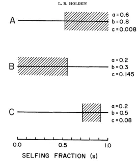
0.52, the two stable noncentral equilibria appear.

However, if either viabilities or recombination fractions different from those used above are chosen, the situation may become more complex. Figure 5b, for example, shows a situation just the opposite of that in 5a. Here the noncentral equilibria, stable for low selfing, disappear if selfing is increased sufficiently. Figure 5c presents an even more complex example: there is no gametic disequi-

-

230 L. R. HOLDEN

A

a

=0.2

b

=0.3

c

=O.

I45

a

=0.2

b

=

0.5

&

~ ~ 0 . 0 8

I l ~ l l l l l l l l

0.0

0.5

I

.o

SELFING

FRACTION

(s)

FIGURE 5a, b, c.-Examples of the three different effects of partial selfing on the maintenance

of gametic disequilibrium. Values of selfing for which there is permanent disequilibrium are indicated by diagonal lines.

librium at low and high selfing values, but for a range of moderate selfing, permanent interlocus association exists.

These three patterns of selfing effects are also illustrated (for the same exam- ples above) in Figure 6, where the critical recombination fraction c, is plotted against the critical selfing fraction so. Figure 6a gives the “intuitive” pattern of

increased selfing resulting in a wider range of linkage values for which gametic disequilibrium exists. I n Figure 6b, just the opposite occurs, and under high outcrossing the looser linkages can maintain gametic disequilibrium. Figure 6c

shows the maximum co value corresponding to an intermediate selfing fraction

(s e 0.85).

It is obvious that with selection, selfing and linkage effects are not analogous. By examining a large number of examples similar to those in Figures

5

and 6, two general patterns of selfing effects on gametic disequilibrium were discovered: ( 1 ) For weak selection against single-heterozygotes (i.e., “large” b ) , an in crease in selfing results in an increase in gametic disequilibrium. Not only is the larger (YI due to an increase in /Yhom.I but also l Y h e t l often increases with the

TWO-LOCUS SELECTION WITH INBREEDING

P

0

0

0

U

a

23 1

0

232 L. R. HOLDEN

for selfing above a “s~fficiently” large value; although this value

is

sometimes very close to one. It is possible that lY( always approaches zero as s approaches one; however, the resolution of the computer solutions was insufficient to allow a determination of this in every case. This decrease in

I

Y

I

with such large s is al- ways due to decreases in

I

Y h e t

I

rather than in

I

Yhonz/. For looser linkages, the in-

crease in disequilibrium with selfing is greater, although the maximum

IY(

and the value of s at the maximum is smaller than with tighter linkage (see Figure 7a).

(2) For strong selection against single-heterozygotes (smaller b )

,

a n increase in the selfing fraction results in a decrease in gametic disequilibrium. This de- crease in

I

Y

I

is characterized by a lower

I

Yhet

I

rather than

I

Yhoml. For the looser linkages, the change in gametic disequilibrium with s is more pronounced; al- though as for large b, the magnitude of

Y

is still greater with tighter linkage (see Figure 7b).

The causes for these phenomena are much too complex to relate in detail, but a general heuristic explanation is straightforward. It is true that selfing, if it re- duces heterozygosity (or more importantly just

H ) ,

will decrease the decay of gametic disequilibrium. This is easily seen by considering the change in Y due to recombination (after selection) :

Y

-

Y

= -2425

-

i)H’,

(28)

where f’ = g‘14/(g’14

+

g J Z 3 ) . Obviously c and H both contribute to the decrease of gametic disequilibrium. If

H

is reduced, the rate of disequilibrium decay is also reduced.

A

b ‘I L A RG E I’

I I

B

IY I

0

0

TIGHT LINKAGE

-

IYI

0

S I

b

“SMALL”

TIGHT LINKAGE

7

I

FIGURE 7a, b.-The typical relationship between the magnitude of gametic disequilibrium

TWO-LOCUS SELECTION WITH INBREEDING 233

Of equal importance, however, is the fact that a low level of double heterozy- gosity can retard the creation of gametic disequilibrium by selection. This is true since the increase in

Yhet

due to selection, i.e.,

(29) also depends upon

H .

(

Yhom

always decreases in magnitude under selection for this model.)

The important question then becomes: which effect predominates, the reduc- tion i n the decay or in the creation of gametic disequilibrium? Apparently, as deduced from the observed patterns, for large b an increase in selfing fraction reduces decay more than buildup and the values of

I

Y

I

at equilibrium are in-

creased. For small b, the opposite occurs.

Lastly, another important consideration of the effects of partial selfing on gametic disequilibrium is the amount of time required for a population to reach an equilibrium. With large selfing fractions, H can be so small that the decay and buildup rate of disequilibrium are also small. This implies that a very large number of generations may be required for the population to reach an equi- librium value of

Y .

For example, with a = 0.2, b = 0.5, c = 0.08, s = 0.99 (i.e.,

as in Figure 5c) and starting with

Y

= 1, it required over 500 generations before

Y decayed to less than 0.001 (over five times longer than with s = 0). It would require a considerable amount of faith to assume that this model could represent a natural population for such a long time.

It

may be more rewarding for future studies to place more emphasis on the dynamics of gametic disequilibrium in a highly selfing population, rather than on just the equilibrium structure.

CONCLUSIONS A N D SUMMARY

This study provides the first solution to a two-locus selection model with partial selfing. AS

such, it forms a bridge between current two-locus, random-mating theory and the results of the purely numerical studies of JAIN and ALLARD (1966). By generalizing two-locus theory for this

specific type of model, I have both verified some of the conclusions of JAIN and ALLARD and have found several new properties.

JAIN and ALLARD (1966) observed that gametic disequilibrium can exist i n this partial selfing model at equilibrium without (additive) epistasis, i.e., with E = 0. In view of the fact

that A ( s ) , not E , is the indicator of disequilibrium potential, this is not surprising. Since it can

be shown that A ( s )

>

A ( 0 ) = e for s

>

0, it is possible to have A ( s )

>

0

>

E . Thus gametic

disequilibrium is possible even with negative epistasis. Obviously, the additive epistasis concept is of little importance without random mating.

234 L. R. H O L D E N

selection for increased recombination. However the claim of CHARLESWORTH, CHARLESWORTH and STROBECK (1977) that these results “suggest that increased levels of selfing on the whole favor a higher intensity of selection for reduced recombination i n constant-environment models with two heterotic loci” is clearly not justified. Such heterotic two-locus models can also display negative disequilibrium potential.

The present study also shows that the common belief in an analogy between greater selfing and tighter linkage to be, in general, unfounded. For some combinations of viabilities, increased selfing can increase o r induce disequilibrium, but the opposite is also possible. By reducing the frequency of double heterozygotes, partial selfing reduces both the decay and the creation of gametic disequilibrium. Only by determining which effect predominates can we specify the fate of interlocus associations.

I have also indicated briefly that under a large selfing fraction, the time required to attain an equilibrium is much longer than under random mating. This is especially relevant when coupled with the fact that gametic disequilibrium can be generated as allelic frequencies change under selection (if D is not exactly zero). Thus, a highly self-fertilizing population observed over time could display a buildup of gametic disequilibrium which would eventually decay, but at a very slow rate. If the eventual decay of disequilibrium to Y = 0 (which is the same as D = 0 in this model) defines no co-adaptation, then it would seem t o be rather difficult to design any short-term experiment to reject the hypothesis that a highly selfed population with Y # 0 is co-adapted. It is conceivable that even a study of 42 generations of a highly selfed (s

>

0.99) plant such as barley (e.g., CLEGG, ALLARD and KAHLER 1972) is not sufficiently long to answer this question.

Finally, I must echo KARLIN’S (1975) warning against “a tendency to offer sweeping con- clusions on the basis of certain particular cases.” Many of the “general” principles given above can be made only by assuming the symmetry and the fairly restrictive values placed on the viabilities. I would expect, for example, from the study of JAIN and ALLARD (1966) and from

single-locus inbreeding theory, that the relaxation of symmetry in two-locus models will make it much more difficult to achieve a stable polymorphic equilibrium with a large selfing fraction. Certainly, the complexity of results will not decrease as the partial selfing model is extended.

I am very grateful to M. T. CLEGG, J. F. CROW, B. S. WEIR, C. STROBECK, J. L. HAMRICK and N. A. SLADE for their helpful comments and criticisms on this manuscript. I wish especially to thank PHILLIP W. HEDRICK f o r his aid in the preparation of the final manuscript.

L I T E R A T U R E CITED

ALLARD, R. W., G. R. BABBEL, M. T. CLEGG and A. L. KAHLER, 1972 Evidence for coadaptation in Avena barbata. Proc. Natl. Acad. Sci. U.S. 69: 3043-3048

ALLARD, R. W., S. K. JAIN and P. L. WORKMAN, 1968 The genetics of inbreeding populations. Advan. Genet. 14: 55-131.

CHARLESWORTH, D., B. CHARLESWORTH and C. STROBECK, 1977 Effects of selfing on selection for recombination. Genetics 86: 213-226.

CHRISTIANSEN, F. B. and M. W. FELDMAN, 1975 Selection in complex genetic systems. IV. Mul- tiple alleles and interaction between two loci. J. Math. Biol. 2: 179-204.

CLEGG, M. T., 1978 Dynamics of correlated genetic systems. 11. Simulation studies of chromo- somal segments under selection. Theoret. Pop. Biol. 13: 1-23.

CLEGG, M. T., R. W. ALLARLI and A. L. KAHLER, 1972 Is the gene the unit of selection? Evi- dence from two experimental plant populations. Proc. Natl. Acad. Sci. US‘. 69: 2474-2478. EWENS, W. M., 1969

FELDMAN, M. W., I. FRANKLIN and G. THOMSON, 1974

Population Genetics. Methuen and Co., London.

TWO-LOCUS S E L E C T I O N WITH I N B R E E D I N G

235

Selection in complex genetic systems. 111. An effect of allele multiplicity with two loci. Genetics 79: 333-347.

Is the gene the unit of selection? Genetics 6 5 : 707-734. Multilocus systems in evolution. Evol. Biol. FELDMAN, M. W., R. C. LEWONTIN, I. R. FRANKLIN and F.

B.

CHRISTIANSEN, 1975

FRANKLIN, I. and R. C. LEWONTIN, 1970 HEDRICK, P. W., S . JAIN and L. HOLDEN, 1978

11: 101-184.

JAIN, S . K., 1968 Simulation of models involving mixed selfing and random mating. 11. Effects

-,

of selection and linkage in finite populations. Theoret. Appl. Genet. 38: 232-242. 1969 Epistasis and linkage in inbreeding populations. Japan. J. Genet. 44: 135-143. JAIN, S. K. and R. W. ALLARD, 1966 The effects of linkage, epistasis, and inbreeding on popu-

KARLIN, S., 1975 General two-locus selection models: some objectives, results and interpretations.

KARLIN, S. and U. LIEBERMAN, 1976 A phenotypic symmetric selection model for three loci,

LEWONTIN, R. C. and K. KOJIMA, 1960 The evolutionav dynamics of complex polymorphisms.

SHIKATA, M., 1963 Representation and calculation of selfed population by group ring. Theoret.

The three locus model with multiplicative fitness values. Genet. Res. 22: 195-200. -, 1976 The three locus model with multiplicative fitness values: the crystallization of the genome, pp. 781-790. In: Population Genetics and Ecology. Edited by

S. K4RLIN and E. NEVO, Academic Press, New York.

TURNER, J. R. G., 1969 Models which help one to understand two-locus polymorphism. Japan.

J. Genet. 44: 131-134.

WEIR, B. S., R. W. ALLARD and A. L. KAHLER, 1972. Analysis of complex allozyme polymor- phisms in a barley population, Genetics 72 : 505-523.

WEIR, B. S . and C. C. COCKERHAM, 1973. Mixed self and random mating at two loci. Genet. Res. 21: 247-262.

WILW, C. and C. MILLER, 1976 A computer model allowing maintenance of large amounts of genetic variability in mendelian populations. 11. The balance of forces between linkage and random assortment. Genetics 82 : 377-399.

YAMAZAKI, T., 1977 The effects of overdominance of linkage in a multilocus system. Genetics

Corresponding editor: B. S. WEIR lation changes under selection. Genetics 53: 633-659.

Theoret. Pop. Biol. 7: 366398.

two alleles: the case of tight linkage. Theoret. Pop. Biol. 10: 334-3M.

Evolution 14: 459-472.

Biol. 5: 142t2r160. STRQBECK, C., 1973

86: 277-236.

A P P E N D I X

Proof that Yhet and Yhom are of the same sign at equilibrium: From (7a),

which implies

236 L. R. HOLDEN

Now as long as H , h

>

0 and s

<

1, then W

>

a. This implies

2W

>

2a

>

( I f s l a , or

( l + s ) a - 2w

<

0 .

Thus,

-

(I-%)

(1fs)a

-2w

Yhet = K ' yhet

.

Yhom =