STILLWELL, CHARLES CALVIN. Urban Hydrology and Low Impact Development:
Exploring New Metrics for Design and Evaluation Across Temporal and Spatial Scales. (Under the direction of Dr. William F. Hunt III).
Low impact development (LID) is a stormwater management strategy that aims to replicate natural hydrologic regimes in urban areas. The goal of LID is to reduce the negative impacts of urbanization – such as flooding, contamination, and stream degradation – to receiving surface waters. Realization of this goal requires widespread LID implementation throughout all the urban areas within a watershed. However, stormwater management design and regulatory enforcement occur at the parcel or subdivision scale, and coordination across the entire watershed is extremely rare. Furthermore, hydrologic processes are complex, dynamic, and difficult to predict, so stormwater control measures (SCMs) are often designed to manage major and infrequent storms rather than the full hydrologic regime. The disconnect between the design and regulatory communities at the sub-watershed scale and the planning and management communities at the watershed scale can hinder the effectiveness of LID towards fulfilling urban stream restoration goals.
In Chapter 1, a suite of long-term hydrologic metrics is introduced (many proposed by others) and their interpretation across spatial scales is discussed with regards to stormwater design and watershed planning. New LID design targets are proposed based on the annual water balance and frequency of runoff events. However, it is noted that many research questions still remain unanswered with regards to LID at the watershed scale.
Chapters 2 and 3 describe subcatchment-scale monitoring and modeling studies
series of scenario analyses that used a process-based model to predict the long-term hydrologic and water quality performance of various SCM types, SCM sizes, and soil characteristics. Infiltration-based strategies reduced significantly greater nutrient loads than harvesting and detention-based strategies in most scenarios, and infiltration basins were more financially effective than all other strategies.
Chapters 4 and 5 outline a data-driven statistical modeling approach to estimate hydrologic metrics across North and South Carolina. Flow data from the USGS streamgage network was used to calculate existing hydrologic metrics in monitored watersheds, then a random forest regression model was developed to predict hydrologic responses as a function of natural and anthropogenic watershed characteristics, such as area, slope, land cover,
precipitation, and soil permeability. Chapter 4 describes the model’s formulation and selection based on predictive ability, interpretability, and its applicability across the study area. The final random forest model used eleven attributes from 283 watersheds to predict three hydrologic responses: annual streamflow volume (NSE = 0.878), annual baseflow index (NSE = 0.884), and number of stormflow pulses per year (NSE = 0.779). In Chapter 5, the model was used to
estimate the importance of each watershed attribute for predicting hydrologic responses, finding that slope, urban land use, and soil permeability were consistently important. Partial dependence analyses were also performed to identify relationships between predictor and response variables, finding that soil permeability, watershed slope, and percent urban land use were consistently important variables for predicting the responses of interest. The model was also used to predict hydrologic responses in more than 50% of the ungaged watersheds across the study area.
Evaluation Across Temporal and Spatial Scales
by
Charles Calvin Stillwell
A dissertation submitted to the Graduate Faculty of North Carolina State University
in partial fulfillment of the requirements for the degree of
Doctor of Philosophy
Biological and Agricultural Engineering
Raleigh, North Carolina 2019
APPROVED BY:
_______________________________ _______________________________ William F. Hunt II Barbara A. Doll
Committee Chair
_______________________________ _______________________________ Emily Z. Berglund Eban Z. Bean
_______________________________ Daniel R. Hitchcock
ii DEDICATION
iii BIOGRAPHY
iv ACKNOWLEDGMENTS
First off, I’d like to thank my friends who have stuck with me throughout my time in grad school. Mike and Josh, it’s hard to believe that we graduated high school 10 years ago, and in that decade you’ve both married and bought houses – I’m planning to occupy those guest bedrooms sometime soon! Dev and Ken, you welcomed me from day one and for that I’m incredibly grateful. Although our first adventures were in and around Philly, we’ve since traveled around the world together; I look forward to our next journey, wherever that may be. Mike, Herrman, and Eric, you were easily the most fun (and reckless) roommates I’ve ever had. Even though we see each other less and less, it’s comforting to know that we will pick up right where we left off as if no time has passed. Dom, Sean, and Katie, I truly believe we were the best ever senior design team to have devoted so much time to a non-existent septic system. I think I actually miss those late nights in the CAD lab, but maybe that’s a side effect of the sleep
deprivation. To every one of you, thank you so much for the fun memories, I cherish everything we have been through together and look forward to staying close for a very long time.
Upon my arrival in Raleigh, I joined up with the other new additions to the Stormwater Team, and together we took Weaver by storm. Well, mostly Kevin took Weaver by storm and we followed his lead. Kevin and Bree, things haven’t really been the same since you left – you should have taken your time, like me and Jeffrey! Or at least found jobs in Raleigh... I must thank all the grad students who preceded me, put the Stormwater Team on the map, and
mentored me through the culture shock of starting grad school. Same goes to the entire extension team, past and present; you’re essential to our success and often underappreciated – thanks Shawn, Andrew, Ryan, Jon, Erin, Sarah, Jeffrey, and Alisha. To Katy, Shane, Katy, and Simon, thanks for making grad school fun and I’m glad we were able to support each other through it all. And sorry if I graded you too hard in BAE 575, I had (and still have) high expectations for you. Last but not least, Bill, thank you for assembling this amazing group of people that I’ve been lucky enough to call my colleagues and friends. This opportunity has meant the world to me, and I appreciate everything you have done to help me succeed. And now that I’m working right down the road, hopefully we will be collaborating again someday soon!
vi TABLE OF CONTENTS
LIST OF TABLES ... viii
LIST OF FIGURES ... xii
Chapter 1: Low Impact Development at the Catchment-scale and Beyond: Technical Challenges, Potential Solutions, and Future Directions ... 1
Urban Stormwater Management: Past and Present ... 1
Low Impact Development: Concerning Spatial Scale ... 3
LID at the Subcatchment-scale ... 3
LID at the Catchment-scale and Beyond ... 6
Bridging the Gap: LID Design Targets for Multiple Scales ... 8
LID Design Targets Based on the Annual Water Balance ... 10
LID Design Targets Based on Rainfall-Runoff Responses ... 13
Additional Metrics for Stream Stability and Ecology ... 16
A Note on Feasibility ... 17
Summary ... 18
Challenges: Catchment-scale LID ... 18
Proposed LID Design Targets ... 18
Future Research Needs ... 19
Dissertation Outline ... 20
Chapter 2: Monitoring Pre- and Post-Development Hydrology and Nutrient Export from a Commercial Development within a Nutrient-Sensitive Watershed in Raleigh, North Carolina ... 22
Introduction ... 22
Methods... 30
Site Description ... 30
Data Collection ... 33
Data Analysis ... 35
Results and Discussion ... 36
Comparison of Pre- and Post-development Rainfall ... 36
Hydrology: Rainfall-Runoff Response ... 37
Hydrology: Annual Volumetric Summaries ... 39
Event-based Pollutant Concentrations ... 40
Annual Pollutant Export Loading Rates ... 44
Limitations ... 46
Summary and Recommendations ... 47
Chapter 3: Modeling the Hydrology, Nutrient Load Reduction, and Cost of Different Stormwater Management Strategies for a Commercial Development ... 50
Introduction ... 50
Methods... 50
Scenario Analyses ... 50
Baseline Model ... 53
Sensitivity Analysis, Calibration, and Validation ... 58
vii
Nutrient Load Reduction Calculations... 63
Statistical Analysis ... 68
Cost Estimates ... 69
Results and Discussion ... 72
Sensitivity Analysis, Calibration, and Validation ... 72
Hydrologic Modeling ... 76
Load Reduction Calculations ... 78
Cost Estimates ... 83
Limitations ... 87
Summary and Recommendations ... 89
Chapter 4: A Random Forests Modeling Approach to Estimate LID Design Targets in North and South Carolina, USA – Part 1: Model Formulation ... 94
Introduction ... 94
Methods... 99
Overview of Random Forest Models ... 99
Data Preparation... 101
Model Configurations ... 105
Modeling Procedure and Analyses ... 107
Results and Discussion ... 108
Predictor Variable Selection ... 108
Distribution of Predictor and Response Variables ... 110
Model Performance ... 118
Predictor Variable Importance ... 127
Summary and Conclusions ... 138
Chapter 5: A Random Forests Modeling Approach to Estimate LID Design Targets in North and South Carolina, USA – Part 2: Model Interpretation, Prediction, and Applications ... 141
Introduction ... 141
Methods... 141
Data Preparation and Model Development ... 141
Explanatory Data Analysis ... 143
Predictions in Ungauged Watersheds ... 144
Example Applications for Watershed Management ... 145
Results and Discussion ... 146
Model Performance ... 146
Explanatory Data Analysis ... 155
Predictions in Ungauged Watersheds ... 163
Example Applications for Watershed Management ... 175
Limitations and Future Directions ... 184
Limitations ... 184
Future Research Opportunities and Potential Model Improvements ... 186
viii LIST OF TABLES
Table 1.1 LID design targets based on annual water balance volumes. Target values are related to the pre-development subcatchment-scale (left) and catchment-scale
(right) equivalents ... 12
Table 1.2 LID design targets based on rainfall-runoff patterns. Target values can be estimated based on their pre-development subcatchment-scale (left) or catchment-scale (right) equivalents ... 15
Table 2.1 Projected population growth in the counties of the Falls Lake watershed by 2035 ... 24
Table 2.2 Land use change in the Falls Lake watershed between 2001 and 2011 ... 25
Table 2.3 Summary of catchment attributes and data collected at each monitoring station .... 34
Table 2.4 Annual rainfall comparison between pre- and post-development monitoring periods. ... 37
Table 2.5 Results of the simple linear regression model ... 37
Table 2.6 Results of the ANCOVA test on event-based rainfall-runoff response ... 38
Table 2.7 Results of the Student’s t-test on runoff threshold ... 38
Table 2.8 Annual volumetric summaries comparing pre- and post-development runoff ... 39
Table 2.9 Median EMCs and statistical tests comparing pollutant concentrations from the pervious areas between pre- and post-development monitoring periods (TSS = total suspended solids, TN = total nitrogen, TP = total phosphorus, TKN = total Kjeldahl nitrogen, ON = organic nitrogen, NH3-N = ammonia, NH2,3-N = nitrate-nitrite, SRP = soluble reactive phosphorus) ... 42
Table 2.10 Median EMCs and statistical tests during post-development monitoring (TSS = total suspended solids, TN = total nitrogen, TP = total phosphorus, TKN = total Kjeldahl nitrogen, ON = organic nitrogen, NH3-N = ammonia, NH2,3-N = nitrate-nitrite, SRP = soluble reactive phosphorus). Sta. 2 was the monitoring point of runoff entering the constructed wetland, Sta. 3 was wetland effluent entering the wet pond, and Sta. 4 was wet pond effluent ... 44
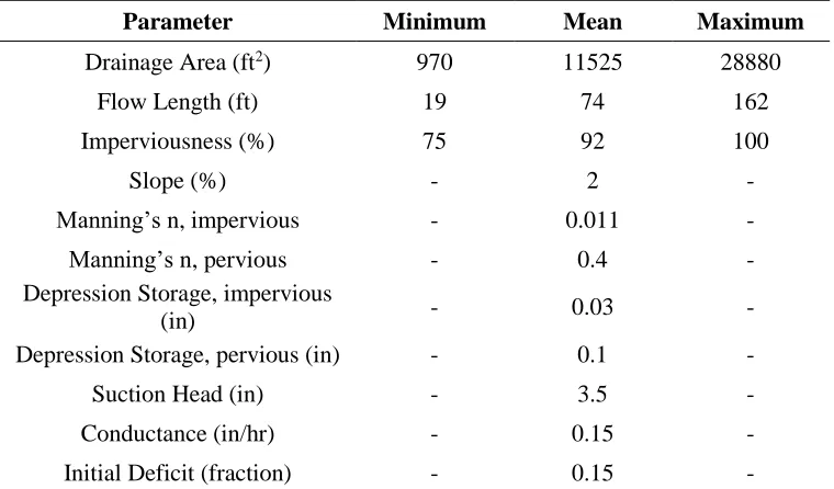
ix Table 3.2 PCSWM input parameter values for the six biofilter subcatchments. Drainage
area, flow length, and imperviousness had unique values for all six biofilters, while the remaining parameters had a standard value applied to all biofilters ... 55 Table 3.3 PCSWM input parameter values for the 33 junctions and conduits. Junction
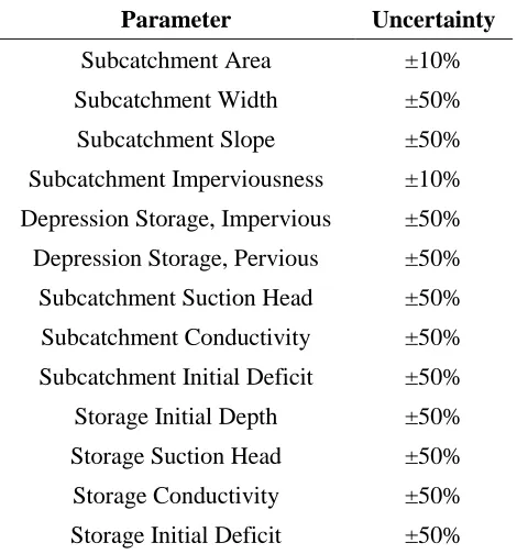
depth, conduit length, conduit slope, and conduit diameter had unique values for all 33 junctions and conduits, while the remaining parameters had a standard value applied to all junctions and conduits ... 56 Table 3.4 Input parameters and uncertainty bounds for the sensitivity analysis and
calibration ... 59 Table 3.5 Wet pond design specifications per the NC Stormwater Design Manual
guidelines. SCM size is indicated across the top; 1.0x is the standard-sized wet pond designed to capture runoff from the 1 inch storm, with other multipliers as indicated (0.5x is half-sized, 2.0x is twice-sized, etc.) ... 61 Table 3.6 Wet ponds with harvesting design specifications per the NC Stormwater Design
Manual guidelines for wet ponds. SCM size is indicated across the top; 1.0x is the standard-sized wet pond designed to capture runoff from the 1 inch storm, with other multipliers as indicated (0.5x is half-sized, 2.0x is twice-sized, etc.) ... 61 Table 3.7 Infiltration basin design specifications per the NC Stormwater Design Manual
guidelines. SCM size is indicated across the top; 1.0x is the standard-sized infiltration basin designed to capture runoff from the 1 inch storm, with other multipliers as indicated (0.5x is half-sized, 2.0x is twice-sized, etc.) ... 62 Table 3.8 Bioretention cell design specifications per the NC Stormwater Design Manual
guidelines. SCM size is indicated across the top; 1.0x is the standard-sized bioretention cell designed to capture runoff from the 1 inch storm, with other
multipliers as indicated (0.5 is half-sized, 2.0x is twice-sized, etc.) ... 63 Table 3.9 Average TN and TP concentrations in rooftop stormwater from monitoring
studies in North Carolina. The median concentration was used for the nutrient load reduction calculations ... 64 Table 3.10 Average TN and TP concentrations in parking lot stormwater from monitoring
studies in North Carolina. The median concentration was used for the nutrient load reduction calculations ... 65 Table 3.11 Average TN and TP EMCs treated by wet ponds from monitoring studies in
North Carolina. The median concentration was used for the nutrient load
x Table 3.12 Average TN and TP EMCs treated by bioretention cells from monitoring studies
in North Carolina. The median TN only considered the bioretention cells with internal water storage (IWS), but the median TP considered all the bioretention cells. The median concentration was used for the nutrient load reduction
calculations ... 66 Table 3.13 Description of treated, bypassed, and lost stormwater volumes for each SCM ... 67 Table 3.14 Nutrient offset rates per credit in North Carolina’s nutrient-sensitive watersheds
(as of 2018) (NC Department of Environmental Quality, 2018c) ... 72 Table 3.15 Results of the sensitivity analysis (NSE = Nash Sutcliffe Efficiency) ... 74 Table 3.16 Results of the Tukey’s range test for TN mass load reductions from each
standard-sized scenario within each in-situ soil infiltration rate ... 82 Table 3.17 Results of the Tukey’s range test for TP mass load reductions from each
standard-sized scenario within each in-situ soil infiltration rate ... 82 Table 3.18 30-year cost estimates for each standard-sized SCM in each in-situ soil
infiltration rate ... 83 Table 3.19 Costs to purchase nutrient offset credits (30-year duration) in North Carolina’s
nutrient-sensitive watersheds, based on 2018 rates (NC Department of
Environmental Quality, 2018c) ... 85 Table 4.1 Watershed and climate attributes considered as predictor variables for inclusion
in the random forest models ... 103 Table 4.2 Criteria for watershed classification based on the level of in-stream structures .... 104 Table 4.3 Land use classifications as defined by the National Wall-to-Wall Anthropogenic
Land Use Trends dataset. These categories were lumped to create the
TOT_URBAN, TOT_URBANFRINGE, TOT_CROP, TOT_PASTURE, and TOT_UNDEVELOPED predictor variables (see Table 4.1) ... 105 Table 4.4 Model configurations consisted of unique combinations of minimum period of
record and input data format ... 107 Table 4.5 Summary of the watershed and climate attributes that were selected for
inclusion in the random forest models ... 109 Table 4.6 Summary of input data for each of the 20 random forest model configurations .... 110 Table 4.7 ANOVA results comparing the effect of in-stream modifiers (Levels) and the
xi Table 4.8 Results of the within-group ANOVA tests comparing the model’s predictive
performance for each response variable (only the statistically significant
differences are shown) ... 125 Table 4.9 The parameters for each best-fit linear model of absolute residual error as a
function of the watershed’s length of record for the L2-1yr-All, L3-1yr-All, and L4-1yr-All random forest models ... 126 Table 4.10 Predictor variable importance when predicting annual streamflow volume.
Importance is listed as increase to root mean squared error, while Δ Rank indicates a relative change in the importance of the predictor variables for the given random forest model configuration ... 128 Table 4.11 Predictor variable importance when predicting annual baseflow index.
Importance is listed as increase to root mean squared error, while Δ Rank indicates a relative change in the importance of the predictor variables for the given random forest model configuration ... 130 Table 4.12 Predictor variable importance when predicting annual stormflow pulses.
Importance is listed as increase to root mean squared error, while Δ Rank indicates a relative change in the importance of the predictor variables for the given random forest model configuration ... 132 Table 5.1 Watershed and climate attributes used as predictor variables in the random
forest model ... 149 Table 5.2 Summary statistics for the root mean squared errors (RMSE) from the 15
repeated L4-1yr-All random forest models. Units match those of the specific
response variables ... 155 Table 5.3 Summary statistics for the Nash-Sutcliffe efficiency coefficients (NSE) from
the 15 repeated L4-1yr-All random forest models ... 155 Table 5.4 Summary statistics for the percent bias (PBias) from the 15 repeated L4-1yr-All
xii LIST OF FIGURES
Figure 1.1 The effect of peak flow mitigation on the discharge hydrograph using detention-based stormwater management strategies (from Roesner et al. 2002) ... 4 Figure 1.2 LID within a hierarchical framework for an urban watershed management
program, adapted from Horne et al. (2017a) ... 9 Figure 2.1 Results of the Final 2016 North Carolina Integrated Water Quality Assessment.
Orange and red represent impairment, red signifying nutrient-related
impairment ... 23 Figure 2.2 Water supply watersheds in North Carolina ... 23 Figure 2.3 Water supply watersheds overlaid by surface waters impaired due to nutrient
loads. Notice the overlap in the urbanized Piedmont region in central North
Carolina ... 24 Figure 2.4 Land use in the Falls Lake watershed. Agriculture (yellow and brown) is
prevalent in the north and west, while urban development (pink and red)
encroaches from the south ... 25 Figure 2.5 Location of the Life Time Fitness facility within the Falls Lake watershed ... 28 Figure 2.6 Life Time Fitness parcel (yellow) in relation to the Falls Lake watershed (blue) ... 29 Figure 2.7 Pre-development (left) and post-development (right). Monitoring stations are
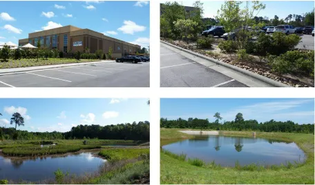
indicated with numbers (see Table 2.3 for details). The watershed ridgeline is marked by the dashed line in the pre-development image. North of the ridgeline is the Falls Lake watershed ... 31 Figure 2.8 Stormwater control measures at the Life Time Fitness facility ... 32 Figure 2.9 Clockwise from top left: building, parking lot biofilter, wet pond, and
constructed wetland ... 33 Figure 2.10 Clockwise from top left: tipping bucket rain gauge, water level logger in wet
pond, water quality sampler at Parking-Runoff, and v-notch weir with bubbler at Pervious-Runoff ... 35
Figure 2.11 Pump status during post-development monitoring ... 40 Figure 2.12 Comparison of pollutant concentrations from pervious areas during pre- and
post-development monitoring periods (TSS = total suspended solids, TN = total nitrogen, TP = total phosphorus, TKN = total Kjeldahl nitrogen, ON = organic nitrogen, NH3-N = ammonia, NH2,3-N = nitrate-nitrite, SRP = soluble reactive
xiii Figure 2.13 Comparison of pollutant concentrations along the suite of SCMs (TSS = total
suspended solids, TN = total nitrogen, TP = total phosphorus, TKN = total Kjeldahl nitrogen, ON = organic nitrogen, NH3-N = ammonia, NH2,3-N =
nitrate-nitrite). Sta. 2 was the monitoring point of runoff entering the constructed wetland, Sta. 3 was wetland effluent entering the wet pond, and Sta. 4 was wet pond effluent ... 43 Figure 2.14 Comparison of estimated annual pollutant export loads from the following
scenarios: pre-development pervious (pink), post-development pervious (green), post-development impervious-then-treated (blue), and total post-development areas (purple) (TSS = total suspended solids, TN = total nitrogen, TP = total phosphorus, TKN = total Kjeldahl nitrogen, ON = organic nitrogen, NH3-N =
ammonia, NH2,3-N = nitrate-nitrite, SRP = soluble reactive phosphorus). The
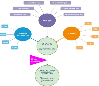
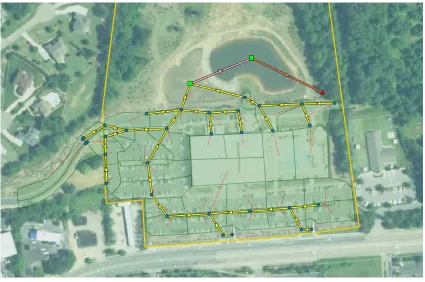
dotted lines in the TN and TP plots represent the Falls Lake Rules limits ... 45 Figure 3.1 Three-factor experimental design to compare annual TN and TP load reductions
between 110 modeled scenarios (or experimental units) ... 51 Figure 3.2 Screenshot of the baseline model in PCSWMM ... 54 Figure 3.3 Conceptual diagram showing the flow of water through a bioretention cell in
PCSWMM ... 57 Figure 3.4 Modeled versus observed weekly flow volumes and the goodness-of-fit statistics
for the uncalibrated baseline model, with 1:1 line shown for clarity (NSE = Nash Sutcliffe Efficiency, RMSE = Root Mean Squared Error, and PBIAS = Percent Bias) ... 73 Figure 3.5 Modeled versus observed weekly flow volumes and the goodness-of-fit statistics
for the calibrated baseline model, with 1:1 line shown for clarity (NSE = Nash Sutcliffe Efficiency, RMSE = Root Mean Squared Error, and PBIAS = Percent Bias) ... 75
Figure 3.6 Modeled versus observed weekly flow volumes and the goodness-of-fit statistics for the baseline model validation, with 1:1 line shown for clarity (NSE = Nash Sutcliffe Efficiency, RMSE = Root Mean Squared Error, and PBIAS = Percent Bias) ... 76 Figure 3.7 Average fates of stormwater from each standard-sized scenario, facetted by
in-situ soil infiltration rate (WP = Wet Pond, Infiltration Basin, BRC =
Bioretention) ... 77 Figure 3.8 Average annual TN mass load reduction (lbs/ac/yr) with 95% confidence
xiv Figure 3.9 Average annual TN mass load reduction (%) with 95% confidence intervals from
each standard-sized scenario facetted by in-situ soil infiltration rate ... 79 Figure 3.10 Average annual TP mass load reduction (lbs/ac/yr) with 95% confidence
intervals from each standard-sized scenario facetted by in-situ soil infiltration rate ... 80 Figure 3.11 Average annual TP mass load reduction (%) with 95% confidence intervals from
each standard-sized scenario facetted by in-situ soil infiltration rate ... 80 Figure 3.12 Estimated 30-year cost to reduce TN loads ($/lbs) with 33.3% uncertainty
bounds from each standard-sized scenario facetted by in-situ soil infiltration rate ... 84 Figure 3.13 Estimated 30-year cost to reduce TP loads ($/lbs) with 33.3% uncertainty
bounds from each standard-sized scenario facetted by in-situ soil infiltration rate ... 84 Figure 3.14 Estimated 30-year cost to reduce TN loads ($/lbs) with 33.3% uncertainty
bounds from each standard-sized scenario facetted by SCM sizing factor ... 86 Figure 3.15 Estimated 30-year cost to reduce TP loads ($/lbs) with 33.3% uncertainty
bounds from each standard-sized scenario facetted by SCM sizing factor ... 87 Figure 3.16 Composite qualitative ratings for each SCM type based on the TN and TP load
reduction potential (left) and the estimated costs to reduce TN and TP loads (right) ... 90 Figure 4.1 Schematic of a simple decision tree (from Hastie et al. 2009) ... 100 Figure 4.2 Schematic describing the formulation and comparison of the random forest
models that were developed in Chapter 4 ... 101 Figure 4.3 Pairwise correlations between full list of predictor variables (left) and reduced
list (right) ... 109 Figure 4.4 Bar charts that demonstrate the different distributions of watershed areas for
each of the 20 random forest model configurations. The panels along the top differentiate the minimum period of record, along the right differentiate the level of in-stream modifiers, and the colors differentiate the data format ... 111 Figure 4.5 Bar charts that demonstrate the different distributions of annual precipitation
depths for each of the 20 random forest model configurations ... 112 Figure 4.6 Density charts that demonstrate the different distributions of annual
xv Figure 4.7 Bar charts that demonstrate the different distributions of urban land use
percentages for each of the 20 random forest model configurations ... 113 Figure 4.8 Bar charts that demonstrate the different distributions of resultant annual
streamflow volumes for each of the 20 random forest model configurations ... 114 Figure 4.9 Density charts that demonstrate the different distributions of resultant annual
streamflow volumes for each of the 20 random forest model configurations ... 115 Figure 4.10 Bar charts that demonstrate the different distributions of resultant annual
baseflow indices for each of the 20 random forest model configurations ... 116 Figure 4.11 Density charts that demonstrate the different distributions of resultant annual
baseflow indices for each of the 20 random forest model configurations ... 116 Figure 4.12 Bar charts that demonstrate the different distributions of resultant annual
stormflow pulses for each of the 20 random forest model configurations ... 117 Figure 4.13 Density charts that demonstrate the different distributions of resultant annual
stormflow pulses for each of the 20 random forest model configurations ... 117 Figure 4.14 Model performance statistics for predicting annual streamflow volume for all
model configurations except the poorly-performing L1-5yr-Mean and L1-15yr-Mean models (NSE = Nash Sutcliffe Efficiency, PBias = Percent Bias, RMSE = Root Mean Squared Error) ... 118 Figure 4.15 Model performance statistics for predicting annual baseflow index for all model
configurations except the poorly-performing L1-5yr-Mean and L1-15yr-Mean models (NSE = Nash Sutcliffe Efficiency, PBias = Percent Bias, RMSE = Root Mean Squared Error) ... 119 Figure 4.16 Model performance statistics for predicting annual stormflow pulses for all
model configurations except the poorly-performing L1-5yr-Mean and L1-15yr-Mean models (NSE = Nash Sutcliffe Efficiency, PBias = Percent Bias, RMSE = Root Mean Squared Error) ... 120 Figure 4.17 Performance statistics for predicting annual streamflow volume for all model
configurations using the annual data format (NSE = Nash Sutcliffe Efficiency, PBias = Percent Bias, RMSE = Root Mean Squared Error) ... 122 Figure 4.18 Performance statistics for predicting annual baseflow index for all model
configurations using the annual data format (NSE = Nash Sutcliffe Efficiency, PBias = Percent Bias, RMSE = Root Mean Squared Error) ... 123 Figure 4.19 Performance statistics for predicting annual stormflow pulses for all model
xvi Figure 4.20 Absolute residual errors and best-fit lines for the L2-1yr-All, L3-1yr-All, and
L4-1yr-All random forest models ... 126 Figure 4.21 Permutation importance results for predicting annual streamflow volumes for
the L4-5yr-Mean, L4-5-yr-Subset, and L4-1yr-All random forest models ... 129 Figure 4.22 Permutation importance results for predicting annual baseflow indices for the
L4-5yr-Mean, L4-5-yr-Subset, and L4-1yr-All random forest models ... 131 Figure 4.23 Permutation importance results for predicting annual stormflow pulses for the
L4-5yr-Mean, L4-5-yr-Subset, and L4-1yr-All random forest models ... 133 Figure 4.24 Permutation importance results when predicting annual streamflow volume for
the L1-1yr-All, L2-1yr-All, L3-1yr-All, and L4-1yr-All random forest models ... 135 Figure 4.25 Permutation importance results when predicting annual baseflow index for the
L1-1yr-All, L2-1yr-All, L3-1yr-All, and L4-1yr-All random forest models ... 136 Figure 4.26 Permutation importance results when predicting annual stormflow pulses for the
L1-1yr-All, L2-1yr-All, L3-1yr-All, and L4-1yr-All random forest models ... 137 Figure 5.1 Street map of North and South Carolina overlaid by the 283 USGS streamgages
used to build the random forest model. The inset in the bottom right (for this figure and all subsequent maps) highlights the urban developed areas indicated by darker gray shading ... 147 Figure 5.2 Map of NHDPlus flowlines in North and South Carolina overlaid by the 283
USGS streamgages used to build the random forest model ... 148 Figure 5.3 Average annual precipitation depths in each watershed. In the random forest
model, annual precipitation depth was reported as a timeseries with unique values for each calendar year, but the above map shows the average values from each watershed's period of record ... 149 Figure 5.4 Average watershed slope for each of the USGS streamgages used in the random
forest model ... 150 Figure 5.5 Average watershed soil permeability for each of the USGS streamgages used in
the random forest model ... 150 Figure 5.6 Percent urban land use for each of the USGS streamgages used in the random
forest model ... 151 Figure 5.7 Total upstream dam storage for each of the USGS streamgages used in the
xvii Figure 5.8 Average annual streamflow volume (inches) at each of the USGS streamgages.
In the random forest model, annual streamflow volumes were reported as a timeseries with unique values for each calendar year, but the above map shows the average values from each watershed's period of record ... 152 Figure 5.9 Average annual baseflow index at each of the USGS streamgages. In the
random forest model, annual baseflow indices were reported as a timeseries with unique values for each calendar year, but the above map shows the
average values from each watershed's period of record ... 153 Figure 5.10 Average annual stormflow pulses at each of the USGS streamgages. In the
random forest model, annual stormflow pulses were reported as a timeseries with unique values for each calendar year, but the above map shows the
average values from each watershed's period of record ... 153 Figure 5.11 Estimated variable importance for predicting annual streamflow volume
according to the permutation importance procedure ... 156 Figure 5.12 Estimated variable importance for predicting annual baseflow index according
to the permutation importance procedure ... 157 Figure 5.13 Estimated variable importance for predicting annual streamflow volume
according to the permutation importance procedure ... 158 Figure 5.14 Partial dependence plots for each predictor variable in combination with annual
streamflow volume. Note that partial dependence relationships can be non-linear and possibly demonstrate threshold responses, but the end behavior may be a
construct of the data as opposed to the physical mechanisms being modeled ... 159 Figure 5.15 Partial dependence plots for each predictor variable in combination with annual
baseflow index ... 161 Figure 5.16 Partial dependence plots for each predictor variable in combination with annual
stormflow pulses ... 162 Figure 5.17 All flowlines in the study area; red lines represent non-streams (such as canals,
ditches, and pipelines) and blue lines represent streams and rivers ... 164 Figure 5.18 All flowlines in the study area; red lines represent out of sample streams and
rivers due to their size (watersheds larger than any of the USGS streamgages used to build the random forest model) ... 164 Figure 5.19 All flowlines in the study area; red lines represent out of sample streams and
xviii Figure 5.20 All flowlines in the study area; red lines represent out of sample streams and
rivers due to dam storage (watersheds with greater normalized dam storage than any of the USGS streamgages used to build the random forest model) ... 165 Figure 5.21 All flowlines in the study area; red lines represent all out of sample streams and
rivers ... 166 Figure 5.22 Gradient of watershed normal annual precipitation depths across all in-sample
NHDPlus flowlines in the study area ... 166 Figure 5.23 Gradient of average watershed soil permeabilities across all in-sample
NHDPlus flowlines in the study area ... 167 Figure 5.24 Gradient of average watershed slopes across all in-sample NHDPlus flowlines
in the study area ... 167 Figure 5.25 Gradient of watershed percent urban land use across all in-sample NHDPlus
flowlines in the study area ... 168 Figure 5.26 Gradient of watershed percent urban fringe land use across all in-sample
NHDPlus flowlines in the study area ... 168 Figure 5.27 Predicted annual evapotranspiration loss volume as a percent of annual normal
precipitation depth for each in-sample NHDPlus flowline within the study area .. 170 Figure 5.28 Predicted annual baseflow volume as a percent of annual normal precipitation
depth for each in-sample NHDPlus flowline within the study area ... 170 Figure 5.29 Predicted annual runoff volume as a percent of annual normal precipitation
depth for each in-sample NHDPlus flowline within the study area ... 171 Figure 5.30 Predicted annual stormflow pulses for each in-sample NHDPlus flowline
within the study area ... 171 Figure 5.31 Coefficients of variation of the predicted evapotranspiration loss volumes for
each NHDPlus flowline from the 15 repeated random forest model runs ... 173 Figure 5.32 Coefficients of variation of the predicted baseflow volumes for each NHDPlus
flowline from the 15 repeated random forest model runs ... 174 Figure 5.33 Coefficients of variation of the predicted runoff volumes for each NHDPlus
flowline from the 15 repeated random forest model runs ... 174 Figure 5.34 Coefficients of variation of the predicted stormflow pulses for each NHDPlus
xix Figure 5.35 Predicted annual evapotranspiration loss volume as a percent of annual normal
precipitation depth for each in-sample NHDPlus flowline within the study area during a prescribed dry year ... 176 Figure 5.36 Predicted annual evapotranspiration loss volume as a percent of annual normal
precipitation depth for each in-sample NHDPlus flowline within the study area during a prescribed wet year ... 176 Figure 5.37 Predicted annual baseflow volume as a percent of annual normal precipitation
depth for each in-sample NHDPlus flowline within the study area during a
prescribed dry year ... 177 Figure 5.38 Predicted annual baseflow volume as a percent of annual normal precipitation
depth for each in-sample NHDPlus flowline within the study area during a
prescribed wet year ... 177 Figure 5.39 Predicted annual runoff volume as a percent of annual normal precipitation
depth for each in-sample NHDPlus flowline within the study area during a
prescribed dry year ... 178 Figure 5.40 Predicted annual runoff volume as a percent of annual normal precipitation
depth for each in-sample NHDPlus flowline within the study area during a
prescribed dry year ... 178 Figure 5.41 Predicted annual stormflow pulses for each in-sample NHDPlus flowline
within the study area during a prescribed dry year ... 179 Figure 5.42 Predicted annual stormflow pulses for each in-sample NHDPlus flowline
within the study area during a prescribed wet year ... 179 Figure 5.43 Estimated LID design targets for stormwater harvesting in the greater
Greensboro-Winston Salem and Raleigh-Durham areas; colors represent the differences in predicted evaporation loss volumes when urban land uses were replace by urban fringe or pasture land uses in the random forest model ... 181 Figure 5.44 Estimated LID design targets for stormwater infiltration or treatment and slow
release in the greater Greensboro-Winston Salem and Raleigh-Durham areas; colors represent the differences in predicted baseflow volumes when urban land uses were replace by urban fringe or pasture land uses in the random forest model ... 182 Figure 5.45 Estimated LID design targets for stormwater runoff reduction in the greater
xx Figure 5.46 Estimated LID design targets for annual pulse reductions in the greater
1 CHAPTER 1 - Low Impact Development at the Catchment-scale and Beyond:
Technical Challenges, Potential Solutions, and Future Directions
Urban Stormwater Management: Past and Present
Continued urbanization has been observed across the globe, and in North America more than 80% of the population already resides in urban areas (United Nations, 2015). Urban land development is expected to continue in the United States; in the southeast, urban areas are expected to replace forested and agricultural land uses (Wear, 2011). Urbanization involves the construction of many impervious surfaces (e.g. roads, sidewalks, parking areas, and buildings) – imperviousness has been identified as a key indicator of urban land use (Arnold and Gibbons, 1996). The introduction of impervious surfaces alters major flow pathways of the hydrologic cycle (as reviewed by Shuster et al. (2005)). The removal of vegetation reduces opportunity for rainfall interception and evapotranspiration, while impervious cover seals the land surface, eliminating infiltration, groundwater recharge, and soil storage. These combined effects, along with soil compaction in lawns and open spaces, result in higher levels of surface runoff in urban areas (Booth and Jackson, 1997). To accommodate for magnified overland flows, cities often utilize stormwater conveyance infrastructure, such as curb-gutter-pipe systems, to efficiently drain excess surface runoff. Impervious surfaces that are drained by stormwater infrastructure and discharge to receiving surface waters are referred to as effective impervious areas or directly connected impervious areas (Shuster et al., 2005).
Alterations to the hydrologic cycle in upland areas have consequent effects in receiving streams. Changes to the flow regime are intuitive, featuring increased stormflow volumes, higher peak flow rates, and flashier flow regimes (Jacobson, 2011). Stormwater can transport a wide variety of constituents from urban areas to receiving streams (Makepeace et al., 1995) and pollutant loads may increase due to the higher stormwater volumes from impervious surfaces (Brabec et al., 2002). Multiple studies have directly linked stream water quality degradation with urban land uses (L. R. Brown et al., 2009; Carpenter et al., 1998; Hatt et al., 2004).
Geomorphologic processes, such as channel deepening, widening, instability, and sediment transport, are often accelerated in urban watersheds (Bledsoe and Watson, 2001; Konrad et al., 2005; Vietz et al., 2016). Urbanization can also affect ecological structure and functions,
2 habitat (Cuffney et al., 2010; Hawley et al., 2016; Konrad and Booth, 2005; Meyer et al., 2005; Walsh and Kunapo, 2009). The conglomeration of hydrologic, geomorphologic, water quality, and ecological impacts resulting from urbanization is referred to as the urban stream syndrome (Paul and Meyer, 2001; Walsh et al., 2005b). These findings have been verified in the Carolinas by multiple research studies (including but not limited to Doll et al. (2002), Lenat and Crawford (1994), Line and White (2007), and O’Driscoll et al. (2010)).
Stormwater management strategies have evolved in response to the symptoms of the urban stream syndrome (Burns et al., 2012). Detention facilities were developed as flood mitigation devices to address magnified peak flows. Although detention-based strategies can successfully reduce peak flows, discharge durations are extended (Booth, 1990; McCuen, 1979) which alters the flow regime of the receiving stream (Roesner et al., 2001) and can increase channel erosion potential (Bledsoe, 2002). Since the 1990s, a variety of stormwater control measures (SCMs) has been introduced as alternatives to detention facilities. These include, but are not limited to, vegetated swales, permeable pavements, bioretention cells (or rain gardens), green roofs, stormwater wetlands, infiltration basins, and street trees (as reviewed by Ahiablame et al. (2012), Dietz (2007), and Eckart et al. (2017)). These devices enhance stormwater
management by promoting infiltration, evapotranspiration, water quality treatment, or any combination of these processes. Harvesting, or reusing stormwater for non-potable demands, has also been suggested as a stormwater management alternative (Mitchell et al., 2007; Walsh et al., 2012); however, harvesting is not common in humid regions where potable water is inexpensive and accessible, such as the Carolinas (Campisano et al., 2017).
3 Low Impact Development: Concerning Spatial Scale
Hydrologic scaling has been the focus of many decades of research, and while advances have been made since the seminal review by Blöschl and Sivapalan (1995), scale relationships remain complex. It has long been understood that runoff and streamflow relationships are dependent upon catchment size, in addition to other watershed characteristics such as soils, land use, and geology (Pilgrim et al., 1982). In urban watersheds, spatiotemporal relations can be further complicated, especially in areas drained by stormwater infrastructure (Kaushal and Belt, 2012).
Throughout this chapter, two spatial scales will be referenced. The subcatchment-scale is defined as an upland drainage area that has not yet discharged to a receiving stream. For this chapter and discussion, the subcatchment-scale in urban areas is generally 1-km2 or less; although smaller drainage areas can create channelized flows in rural catchments, these headwater streams are often replaced by subsurface drainage infrastructure in urban areas (Elmore and Kaushal, 2008). The catchment-scale refers to larger upland areas and the stream channels that drain them; thus, the catchment-scale includes all upland and in-stream hydrologic processes. The following sections will identify the functional hydrologic differences between the subcatchment and catchment-scales with particular emphasis on LID strategies. Another
distinction at these scales are the key drivers and involved parties; LID sites are designed by engineers and regulated by municipalities at the subcatchment-scale, while catchment-scale LID is driven by long-term watershed planning efforts. Collaboration between these groups is rare, and such a siloed approach has implications for the advancement of widespread LID
implementation and evaluation. LID at the Subcatchment-scale
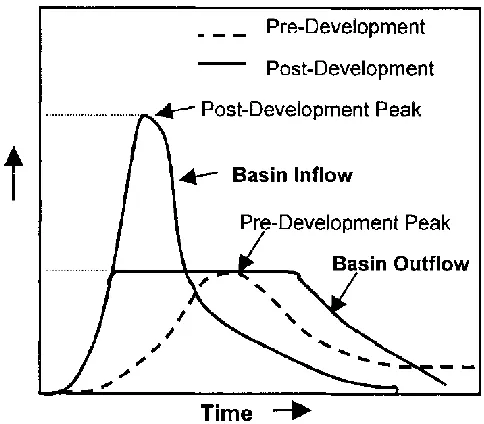
4 Secondly, how is pre-development hydrology defined numerically? Hydrologic patterns are complex and dynamic, and single metric approaches often create unintended consequences. For illustrative purposes, the shortcomings of the traditional flood mitigation approach are used as an example. Flood mitigation strategies require post-development peak discharge rates to not exceed pre-development estimates, based on a design storm or set of design storms. As shown in Figure 1, even when peak flows are successfully controlled, the resultant hydrograph does not match the pre-development condition; longer durations of discharge can increase erosion potential in the receiving stream (Bledsoe, 2002; Roesner et al., 2001). Another shortcoming of the flood mitigation approach is that design storms are selected to represent extreme events while the remainder of the long-term hydrologic record is ignored.
Figure 1.1 - The effect of peak flow mitigation on the discharge hydrograph using detention-based
stormwater management strategies (from Roesner et al. 2002).
New stormwater management strategies are more comprehensive than the flood
mitigation approach; however, the full hydrologic regime is rarely addressed. In North Carolina, the Department of Environmental Quality offers two stormwater management options: the Runoff Treatment option and the Runoff Volume Match option (NC Department of
5 systems. Although a variety of SCMs are available, detention-based strategies are still permitted; hence, problems associated with the flood mitigation approach, like land degradation, can persist. The Runoff Treatment strategy is designed to improve water quality but does not address the flow regime (in Burns et al. (2012), this is referred to as the load-reduction approach). While these regulations can improve conditions in the receiving stream, they do not comprehensively counteract the effects of the urban stream syndrome (Dhakal and Chevalier, 2016; Petrucci et al., 2013).
The Runoff Volume Match option requires that the annual runoff volume does not increase by more than 10% following development (or 5% in high priority areas). The Runoff Volume Match option is essentially North Carolina’s naming convention for LID. By replacing design storms with annual hydrologic volumes, the Runoff Volume Match option attempts to integrate flow regime control into stormwater management. There are no specifications whether stormwater should be infiltrated or harvested, as long as it is not in the form of runoff;
consequently, detention-based SCMs are discouraged. Although the Runoff Volume Match option provides an opportunity to implement LID strategies, it is not a requirement. As a result, adjacent land development projects are permitted to implement vastly different stormwater management strategies – one with an end-of-pipe wet pond, another with a suite of source control SCMs.
6 LID at the Catchment-scale and Beyond
As spatial scales increase so does complexity. Hydrologic flow paths are vastly different beyond the subcatchment-scale. LID strategies attempt to mimic the pre-development volumes of annual infiltration, evapotranspiration, and surface runoff. Infiltrated stormwater is assumed to be “lost” from the water balance even though its fate is unknown; potential flow paths include groundwater recharge, shallow subsurface flow, reemergence as overland flow, or
evapotranspiration from the soil column (Cizek and Hunt, 2013). Subsurface flow paths in urbanized areas are even more uncertain due to buried infrastructure and modified soils (Bhaskar et al., 2016a; Bonneau et al., 2017). Studies investigating the relationships between different SCM types, LID, and urban baseflow have demonstrated complex interactions and unpredictable responses (Bhaskar et al., 2016b; Bonneau et al., 2018b, 2018a; Hamel et al., 2013; Jefferson et al., 2015). Although stormwater infiltration is almost always preferred over untreated discharge, the supposition that infiltrated water is “lost” from the hydrologic regime is oversimplified and can lead to unintended consequences in the receiving stream (Bhaskar et al., 2016b). The only guaranteed mechanisms to eliminate water from reaching any stream is through
evapotranspiration. Harvesting and reuse can eliminate water from a specific receiving stream because stormwater is redirected to the wastewater network, treated, and released to a larger stream or river.
Another widely recognized hydrologic scaling issue is the variable source area concept, first introduced by Hewlett and Hibbert (1965), which states that overland flow at the hillslope (subcatchment-scale) does not always contribute overland flow to the receiving stream. Instead, the drainage area that contributes overland flow to the stream depends on precipitation patterns (depth, intensity, duration) and watershed characteristics (slope, soils, land cover). The
complexity of flow paths from variable source areas increases with spatial scale. Urban variable source areas are often expanded when directly connected impervious surfaces drain to receiving streams (Miles and Band, 2015). LID strategies must understand that the hydrologic effects of land development will be magnified compared to pre-development conditions when the receiving stream is directly connected to drainage infrastructure.
7 aspects of the flow regime, many of which are relevant in the fields of geomorphology and ecology (Eng et al., 2017; Olden and Poff, 2003). Flow metrics can also be used to detect hydrologic alteration and provide guidance towards restoring natural flows (Poff et al., 2010; Richter et al., 1996). Diffuse upland modifications, including urbanization, are widely
recognized as a source of hydrologic alteration (Allan, 2004; Horne et al., 2017b). Current LID implementations at the subcatchment-scale rarely consider specific flow pattern alterations in the receiving stream. The integration of flow metrics into the LID design and regulatory process is an area of unexplored research.
Two major challenges impede the quantification of pre-development hydrologic
conditions at the catchment-scale. One, observed data are rarely available; two, most catchments are already disturbed. For these reasons, models are almost always needed to estimate pre-development hydrologic regimes. In North Carolina, simple empirical equations (such as the NRCS curve number method, (US Department of Agriculture, 1986)) are often used in the design community to estimate infiltration, evapotranspiration, and runoff at the subcatchment-scale (NC Department of Environmental Quality, 2017). However, these methods are mostly invalid beyond the subcatchment-scale. Instead, process-based models can be developed for catchment-scale hydrologic estimations, but these models often lack observed data for calibration and validation. Data from reference watersheds can also be utilized, but it has been demonstrated that seemingly similar watersheds still have dissimilar hydrologic responses (Oudin et al., 2010). Innovative modeling approaches, such as statistical data-driven models, are emerging as
alternatives to estimate pre-development hydrology in ungauged watersheds (Al-Amin and Abdul-Aziz, 2013; Murphy et al., 2013).
8 studies in a variety of regions, watershed typologies, and SCM combinations. Although many catchment-scale LID modeling studies have been conducted (also reviewed by Jefferson et al. (2017)), their validity is difficult to gauge without monitoring data to validate model
performance.
The majority of this chapter mainly discusses technical challenges impeding widespread LID implementation and evaluation, but societal challenges are also important to consider. Although LID is mainly considered a stormwater management strategy, at the catchment-scale is should also be viewed as a form of urban flow regime management (Bernhardt and Palmer, 2011; Walsh et al., 2005a). The determination of restoration target conditions at the catchment-scale must consider scientifically and socially acceptable management targets, which requires input from many stakeholders (Smith et al., 2016). In contrast to the subcatchment-scale,
coordinated efforts throughout the catchment, and sometimes between multiple jurisdictions, are required to align management goals. LID strategies are only as effective as their level of
implementation throughout a watershed, which poses a challenge towards evaluating LID effectiveness at broader spatial scales. A full review of non-technical obstacles preventing
widespread LID implementation is out of the scope of this chapter and has been comprehensively reviewed by others (Dhakal and Chevalier, 2017; Roy et al., 2008).
Bridging the Gap: LID Design Targets for Multiple Scales
Widespread LID implementation and evaluation are hindered by hydrologic scaling issues and a disconnect between the design, regulatory, planning, and research communities. At the subcatchment-scale, the design engineer’s job is to comply with regulations while
9 management at the subscale with urban flow regime management at the catchment-scale.
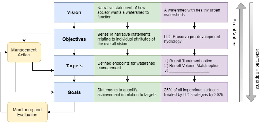
A hierarchical framework of the LID philosophy can help to identify scaling issues. As demonstrated in Horne et al. (2017a), a vision related to water management (or any
environmental problem) can be broken into three increasingly specific categories: objectives, targets, and goals (Figure 2). For this discussion, LID will be considered an objective within a broader vision statement for a city or watershed.
Figure 1.2 - LID within a hierarchical framework for an urban watershed management program, adapted
from Horne et al. (2017a).
10 Goals are even more specific, requiring a timeline with quantifiable assessment. In the LID context, a goal might specify what percentage of impervious surfaces in a catchment should be treated by LID strategies by a certain year (Hopkins et al., 2018). Goals are important for understanding the temporal constraints of catchment-scale LID evaluation; LID effectiveness will change as a function of time and the degree of implementation.
The remainder of this chapter presents potential targets for catchment-scale flow regime management that could be integrated into the LID designs and regulations. Proposed targets should span spatial scales; in other words, each metric must have some physical meaning at the subcatchment-scale (a target for LID design) and at the catchment-scale (an expected response in the receiving stream). It should be noted that the proposed flow regime metrics are mostly
unverified, and additional research is needed to confirm their validity across spatial scales and in a variety of regions and watershed typologies. Also, there are numerous non-technical obstacles to overcome before catchment-scale LID implementations can be properly assessed; flow regime metrics only provide potential solutions to the aforementioned technical challenges.
LID Design Targets Based on the Annual Water Balance
The most common LID guidance is to match the pre-development annual runoff volume. While runoff reduction is the primary stormwater management concern at the subcatchment-scale, a more thorough assessment of catchment flow paths and fates may better protect the receiving stream. Metrics based on the catchment water balance are already widely accepted in the research community (Askarizadeh et al., 2015; Walsh et al., 2012); in fact, mimicking the pre-development water balance is listed as one of the main “principles for urban stormwater management to protect stream ecosystems” in Walsh et al. (2016). Despite widespread
recognition of its importance in the research community, it is rarely employed as a target for LID design (although annual runoff volumetric targets are very similar).
The pre-development subcatchment annual water balance is defined as follows:
P = ETsubcatchment + I + Rpervious
where P represents annual precipitation volume, ETsubcatchment represents annual
evapotranspiration volume, I represents infiltration volume, and Rpervious represents overland
11 new elements to the subcatchment water balance equation. The post-development LID
subcatchment annual water balance is defined as follows:
P = ETsubcatchment + I + Rpervious + Rharvested + Rfiltered + Roverflow+ 𝑅𝑖𝑚𝑝𝑒𝑟𝑣𝑖𝑜𝑢𝑠
where Rharvested represents the volume of harvested runoff, Rfiltered represents runoff volume
filtered through an SCM and discharged to the drainage network, and Roverflow represents runoff
volume intended for SCM treatment that exceeded design capacity, and Rimpervious represents
runoff volume directly discharged to the drainage network from impervious surfaces. To avoid using detention-based SCMs, such as wet ponds, Rfiltered requires stormwater to pass through
some filtration mechanism (bioretention cell, permeable pavement, green roof, etc.). Stormwater that percolates through SCM filter media and exfiltrates to the soil would be considered I, while stormwater percolates through SCM filter media and discharges to the drainage network via underdrain would be considered Rfiltered.
Most existing LID guidelines, including the Runoff Volume Match option in North Carolina, aim to decrease stormwater discharge to the drainage network by promoting infiltration-based SCMs as the main mechanism for runoff reduction. This approach is not always feasible, especially if new developments are highly impervious or located in areas with high water tables or low permeability soils. The third component of the water balance,
evapotranspiration, is often ignored, despite its significance at the catchment-scale. The catchment annual water balance is defined as follows:
P = ETcatchment + Qbaseflow + Qstormflow
where ETcatchment represents annual evapotranspiration volume, Qbaseflow represents the baseflow
component of the annual streamflow volume, and Qstormflow represents the stormflow component
of the annual streamflow volume. This definition assumes that the change in storage is approximately zero over the course of a full year (which may not be valid sub-annually) and lumps all “losses” (canopy interception, deep percolation, etc.) into the evapotranspiration term. The distinction between Qbaseflow and Qstormflow is somewhat subjective; for this discussion,
pre-development Qbaseflow is defined as flow reaching the stream via subsurface flow paths and
pre-development Qstormflow is overland surface flow or shallow interflow. In a post-development
catchment, Qbaseflow is considered any inter-event flow; subsurface flowpaths are highly uncertain
12 any additional streamflow volume during storm events; urban stormflow pathways may include drainage infrastructure, overland conveyances, or preferential subsurface conduits.
Table 1.1 - LID design targets based on annual water balance volumes. Target values are related to the
pre-development subcatchment-scale (left) and catchment-scale (right) equivalents.
Pre-development
Subcatchment LID Design Targets
Pre-development Catchment
ETsubcatchment ≈ ETsubcatchment + Rharvested ≈ ETcatchment
I ≈ I + Rfiltered ≈ Qbaseflow
Rpervious ≈ Rpervious + Roverflow + Rimpervious ≈ Qstormflow
Table 1.1 shows the post-development LID design targets that aim to mimic the pre-development water balance at both spatial scales. As shown, each of the additional elements in post-development LID subcatchment equation (Rharvested, Rfiltered, Rbypassed, and Rimpervious) have
been allocated to an existing component of the pre-development water balance.
The LID design targets based on the annual water balance have two major differences from North Carolina’s Runoff Volume Match option. First, a volumetric stormwater harvesting target is explicitly defined as the evapotranspiration deficit following land development.
Stormwater harvesting, although uncommon in North Carolina, is typically utilized to supplement irrigation or internal uses. Irrigated stormwater is assumed to infiltrate or evapotranspire during inter-event periods (as long as the irrigation schedule and rate are appropriately selected), which exactly mimics evapotranspiration loss. Internally reused stormwater is assumed to enter the wastewater stream, which is likely to be treated and
discharged in a different catchment. Under either scenario, harvested stormwater is lost from the local water balance and does not contribute to the receiving stream. Second, all filtered
13 The water balance targets previously listed still assume multiple scaling relationships. Notably, ETsubcatchment, I, and Rpervious are assumed to correspond with ETcatchment, Qbaseflow, and
Qstormflow (respectively) and the validity of these assumptions has already been discussed.
Bonneau et al. (2018b) further illustrated the complexities of urban flow paths – some infiltrated stormwater was evapotranspired downslope, while some was conveyed out of the catchment via preferential subsurface flow paths. Specific interactions between subcatchment hydrology and the receiving stream will vary by region, watershed typology, urban density, and stream proximity (Miles and Band, 2015). Another assumption is that stormwater volumes filtered through an SCM will mimic the timing of inter-event flow in the receiving stream. A few studies have compared the discharge patterns of bioretention cells to forested reference streams and have demonstrated similarities (DeBusk et al., 2011; Olszewski and Davis, 2013). Further research is needed to confirm the validity of the assumptions listed above; that being said, the proposed targets in Table 1.1 are expected to preserve pre-development hydrologic patterns better than existing runoff reduction targets because they account for multiple hydrologic pathways and the eventual fate of stormwater.
To employ the targets listed in Table 1.1, estimates of the pre-development water balance are necessary, either from the subcatchment or catchment-scale. As previously discussed,
modeling methods at these scales are not consistent. While simple empirical modeling equations such as the curve number method would be preferred in the design community, there are two shortcomings. First, these empirical equations were developed for event-based predictions, not for predicting annual water balances (although they have been utilized for such predictions, such as the NC Stormwater Design Manual [2017]). Second, these equations are not based on the flow regime from the receiving stream. For these reasons, predictions based on the catchment-scale water balance are preferred from a scientific perspective; however, advanced modeling
techniques will be needed. Additional research on the prediction of pre-development annual water balances at different spatial scales is needed.
LID Design Targets Based on Rainfall-Runoff Responses
14 infiltration rate, forcing water to flow laterally over the surface. Since impervious surfaces
eliminate infiltration, essentially all precipitation events cause Horton overland flow in urban areas (Miles and Band, 2015); thus, its applicability as a stormwater design target is limited. Dunne overland flow occurs when precipitation volume exceeds subcatchment storage capacity and water ponds and flows above the surface. Dunne overland flow is sometimes referred to as “fill and spill” runoff – the fill and spill concept can be used to form LID design targets.
At the subcatchment-scale, the precipitation volume retained prior to runoff is referred to as initial loss, initial abstraction, or the runoff threshold (runoff threshold is used herein). The pre-development runoff threshold can be defined as follows:
RT = Sdepression + Ssoil
where RT represents the runoff threshold, Sdepression represents depression storage, and Ssoil
represents soil storage. Both Sdepression and Ssoil are dependent upon antecedent rainfall, so RT it is
not a static value (although it can be estimated from local precipitation patterns). The post-development runoff threshold can be defined as:
RT = Sdepression+ Ssoil + SSCM
where SSCM represents the storage capacity of on-site SCMs, which is again dependent upon
antecedent rainfall. Impervious surfaces seal underlying soils and generally ensure positive drainage, so Sdepression and Ssoil are both greatly reduced in urban areas (Miles and Band, 2015).
Measures of RT account for a subcatchment’s retention capacity, not storage in detention facilities. Water stored as Sdepression or Ssoil are depleted between rainfall events by either
infiltration or evapotranspiration and do not discharge to the receiving stream as stormflow. Therefore, SSCM should only include storage volumes that can be diminished via harvesting,
infiltration, or evapotranspiration between storm events (in other words, temporary storage in detention facilities is invalid). Retention capacity has been proposed as a LID design target within the research community (Walsh et al., 2009) but has not gained traction as a regulation.
15 accounts for all hydrologic interactions that may occur between the upland areas and the
receiving stream; in other words, runoff on a hillslope does not always reach the stream as overland flow. In urban catchments variable source areas expand and watershed capacitance reduces, both due to directly connected impervious surfaces and drainage infrastructure (Miles and Band, 2015). Because of the aforementioned complications, exact physical estimates of watershed capacitance are difficult to quantify; instead, hydrograph spikes of an arbitrary magnitude are used to define runoff events, such as 3 times the median flow (Eng et al., 2017; Olden and Poff, 2003). However, most of these flow metrics are intended to define flood pulses, not all flows with runoff contributions.
Table 1.2 shows two post-development LID design targets that aim to mimic pre-development rainfall-runoff patterns. The first is based on the estimated runoff threshold and watershed capacitance volumes; however, as previously noted, estimates of runoff threshold and watershed capacity are highly variable and difficult to quantify. An alternative approach is to count the number of runoff events (spikes in the hydrograph) per year, which accounts for antecedent rainfall variability and may be easier to estimate than the volume based targets.
Table 1.2 - LID design targets based on rainfall-runoff patterns. Target values can be estimated based on
their pre-development subcatchment-scale (left) or catchment-scale (right) equivalents.
Pre-development
Subcatchment LID Design Targets
Pre-development Catchment
Volume-based → Sdepression + Ssoil ≈ Sdepression + Ssoil + SSCM ≈ Capacitance
Frequency-based → # Dunne / year ≈ # SCM bypasses / year ≈ # spikes / year
16 Neither approach is devoid of hydrologic scaling issues. As described by the variable source area concept, runoff in an upland subcatchment may not even reach the receiving stream, so estimated pre-development runoff threshold volumes and watershed capacitance will never perfectly align. Similar challenges limit the frequency-based approach, because a spike of specific magnitude in a streamflow hydrograph is controlled by many factors, not just upland runoff. Additional research is needed to compare subcatchment and catchment-scale pre-development runoff patterns, but relationships may be too heterogeneous for application across watersheds and regions.
There are no simple empirical equations to estimate the runoff threshold or the frequency of Dunne overland flow events at the subscale. Instead, pre-development catchment-scale estimates may be easier to calculate, but only if streamflow is monitored or estimated. Further research is needed to determine the best modeling approaches for predicting pre-development runoff responses at either spatial scale.
Additional Metrics for Stream Stability and Ecology
Many efforts to assimilate flow regime control into stormwater management and watershed hydrology have been researched and advocated ever since the recognition of detention-based shortcomings. However, most of these studies approached the problem by altering discharge patterns rather than adjusting on-site stormwater management strategies. Some example studies are discussed in brief; however, the necessity of geomorphologic or ecologic metrics may be greatly reduced if the previously proposed LID design metrics are utilized. Flow has been coined the “master variable,” meaning that nearly all water quality, geomorphologic, or ecological consequences are somehow related to hydrologic alteration (Poff et al., 1997).
Because the proposed LID design targets aim to minimize hydrologic alteration, many consequential impacts may be mitigated; in other words, these LID design targets address the causes, not the symptoms, of the urban stream syndrome.
17 local conditions were needed to inform the optimal designs. Tillinghast et al. (2011) also used modeling approaches to calculate three stormwater management metrics for stream stability in central North Carolina: unit critical discharge, annual allowable erosional hours, and annual allowable volume of eroded bedload. Hawley and Vietz (2016) demonstrated the importance of critical discharge over 2-year peak flows and how critical discharge targets can be integrated into stormwater management. Metrics based on flow duration curves have also been suggested. Vogel et al. (2007) first introduced the terms ecodeficit and ecosurplus, which measure differences between pre-development and disturbed flow duration curves and can be used to identify alterations to low and high flows. Stein et al. (2012) advocated the flow duration control box which targets a specific portion of the flow duration curve where variations should be
minimized. The aforementioned approaches only represent a small portion of stormwater
management vis-a-vis stream stability studies, and research continues to explore new metrics for geomorphologic management.
Another area of hydrologic research is the determination of ecological responses to hydrologic alteration (Bunn and Arthington, 2002; Poff and Zimmerman, 2010) and the selection of ecologically relevant metrics as restoration targets (Mazor et al., 2018). A full review of these studies is outside of the scope of this chapter; instead, a few notable examples are presented. Hawley et al. (2016) demonstrated how critical discharge is correlated with benthic disturbance and ecological degradation. Anim et al. (2019) developed three ecologically relevant metrics that could be used to guide stormwater design: benthic mobilization, hydraulic diversity, and
retentive habitat availability. Some researchers predict a suite of ecological flow metrics for classification and management purposes (Eng et al., 2017; Olden and Poff, 2003). Many ecologically relevant hydrologic metrics are based on seasonal patterns, which are difficult to design for using passive stormwater systems. The emergence of real-time control systems may help integrate ecological metrics into stormwater design and could be used at the catchment-scale to prevent superposition of peak flows in the receiving stream (Kerkez et al., 2016). A Note on Feasibility