Thermal Modeling and Simulation of Electron Beam Melting for Rapid Prototyping on Ti6Al4V Alloys.

(1)

ABSTRACT

NEIRA ARCE, ALDERSON. Thermal Modeling and Simulation of Electron Beam Melting for Rapid Prototyping on Ti6Al4V Alloys. (Under the direction of Dr. Jerome Cuomo.)

To be a viable solution for contemporary engineering challenges, the use of titanium alloys in a wider range of applications requires the development of new techniques and processes that are able to decrease production cost and delivery times. As a result, the use of material consolidation in a near-net-shape fashion, using dynamic techniques like additive manufacturing by electron beam selective melting EBSM represents a promising method for part manufacturing. However, a new product material development can be cost prohibitive, requiring the use of computer modeling and simulation as a way to decrease turnaround time.

(2)

analysis (IR-Thermography), laser diffraction, liquid and gas pycnometry using mercury and krypton adsorption respectively.

This study was followed by the review of complementary strategies to simulate the temperature evolution during the EBSM process, using a finite element analysis package called COMSOL Multiphysics. Two alternatives dedicated to representing a moving heat source (electron beam) and the powder bed were developed using a step-by-step approximation initiative. The first method consisted of the depiction of a powder bed discretized on an array of domains, each one representing a static melt pool, where the moving heat source was illustrated by a series of time dependant selective heating and cooling steps. The second method consisted of the solution of a prescribed domain, where each powder layer is discretized by an individual 3D element and the heat source is represented by a 1D element displaced by a temperature-coupling extrapolation routine. Two validation strategies were presented here; the first was used to confirm the accuracy of the proposed model strategy by setting up a controlled experiment; the second was used to validate the post-processing data obtained by the simulation by comparison with in-situ measured EBSM process temperature.

(3)

(4)

Thermal Modeling and Simulation of Electron Beam Melting for Rapid Prototyping on Ti6Al4V Alloys

by

Alderson Neira Arce

A dissertation submitted to the Graduate Faculty of North Carolina State University

in partial fulfillment of the requirements for the Degree of

Doctor of Philosophy

Materials Science and Engineering

Raleigh, North Carolina 2012

APPROVED BY:

__________________________________________________ Dr. Jerome Cuomo

Advisory Committee Chair

_____________________________________________ Dr. John S. Strenkowski

Committee Member

__________________________________________________ Dr. Michael Rigsbee

Committee Member

_________________________________________________ Dr. Jonathan Bohlmann

(5)

ii

DEDICATION

This dissertation is dedicated to my grandmother Rosita for her kindness and devotion while teaching me the value of persistence and dedication; to my mother Elizabeth for her endless and unconditional support; to my wife Lilian for her encouragement, love and friendship and to my daughter Kristen for bringing me happiness every day of my life.

(6)

iii

BIOGRAPHY

(7)

iv manufacturing, where he made his contribution on solid lubricant surfaces produced by Laser Engineered Net Shaping and later by the modeling and simulation of Electron Beam Melting processes, the later research led by Dr. Jerome Cuomo at the Institute of Maintenance Science and Technology in North Carolina State University. Additional activities during graduate school includes the use of atmospheric plasmas for digital micro fluidics applications on electro wetting on dielectric devices as well as destructive and non-destructive characterization of metal, polymers and composite materials.

(8)

v

ACKNOWLEDGMENTS

For their guidance and mentorship, I would like to thank Dr. Jerome Cuomo, Dr. Denis Cormier, Dr. Dick Guarnieri, Dr. John Strenkowski, Dr. Michael Rigsbee and Dr. Jonathan Bohlmann.

For their financial support I would also especially like to thank the Laboratory for Integrated Manufacturing Science and Technology (LIMST) at NC State University as well as the U.S. Department of Defense, through the Strategic Environmental Research and Development Program (SERDP) - Project No. WP-1762, the Navy Small Business Innovation Research - Project No. N102-166-0752 and Bennett Aerospace Inc.

For their group effort at LIMST - MSE, to Darin Thomas, Shaphan Jernigan, James Mulling, Dr. Steven Hudak and Dr. Roger Sanwald.

For their invaluable technical support on this dissertation to Dr. Ilir Beta, Robert Campbell and Bob Fidler at NETZSCH Instruments of North America, LLC; Joel Mancuso and Rich Fiore at Gatan Inc.; Steven Neptun, Luke Hunter and Naomi

(9)

vi At NC State University I would like to extend my gratitude to Dr. Christopher Bobko from CCEE, as well as Tim Horn and Dr. Ola Harrison at ISE.

To my dear friends Dr. Federico Sequeda, Dr. Thomas Scharf, Dr. Nalin Kumar, Dr. Christopher Oldham, Dr. Theodore Winger, Victor Prince, Brad Hartman, Matthew King, Ty Wang, Dr. Anthony McWilliams and Dr. Jackson Thornton.

(10)

vii

LIST OF FIGURES

Figure 1.1. EBSM (ARCAM A-2) System Illustration ...11

Figure 2.1. Laser diffraction technique (adapted from [84])...36

Figure 2.2. Wet dispersion system Cilas 1800 using a 5gms sample size and obscuration of 1.2% ...37

Figure 2.3. Dry dispersion system Malvern 2000 using a 250grams sample size and obscuration values of 3.91% ...38

Figure 2.4. Axial chromatism operation principle (adapted from [85]) ...40

Figure 2.5. Image of solid Ti4Al4V (left) and sintered TiAl4V (right) used for 3D roughness analysis ...41

Figure 2.6. Micro-CT Scan setup ...43

Figure 2.7. Sample orientation illustration used for thermal analysis on Ti6Al4V solid parts ...47

Figure 2.8. Laser flash operation principle ...52

Figure 2.9. Half time temperature pulse calculation ...53

Figure 2.10. Nicolet 8700 FT-IR System ...56

(14)

xi Figure 2.12. Emissivity sample setup: a. EBSM processed Ti6Al4V

holder; b. Ti6Al4V powder; c. Solid Ti6Al4V partially

coated with graphite; d. Sintered Ti6Al4V powder; e. Powder and partially graphite coated rough Ti6Al4V

solid; f. Side view image during sample heating. ...58 Figure 2.13. FTIR Analysis on Quartz window ...59 Figure 2.14. Viewport correction setup ...60 Figure 2.15. Thermal Camera Calibration with black body source

behind Quartz window...61 Figure 2.16. EBSM Powder Raking System...63 Figure 2.17. Cube built image (PREP powder) after being processed

by EBSM. Sample is embedded in PREP powder

material. ...63 Figure 2.18. EBSM processed Ti6Al4V cube sample from PREP

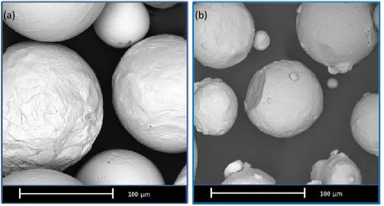
powder ...64 Figure 3.1. SEM images PREP (left) GA (right) ...68 Figure 3.2. Ti6Al4V PREP powder contact surface SEM image ...69 Figure 3.3. Computed tomography images. Reconstructed 2D slices

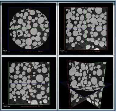
from sintered Ti6Al4V (GA) powder. Each of the quadrants represents a different orthogonal virtual slice. The colored lines correspond to slices with the

same border color. ...71 Figure 3.4. Porosity on (GA) sintered material ...72 Figure 3.5. 3D volume rendering on Ti6Al4V sintered GA powder

(15)

xii Figure 3.6. Reconstructed 2D slices from sintered Ti6Al4V PREP

powder. Each of the quadrants represents a different orthogonal virtual slice. The colored lines correspond to

slices with the same border color. ...74 Figure 3.7. Porosity view on PREP powder material ...75 Figure 3.8. PREP powder 3D rendering ...76 Figure 3.9. 3D Image rendering for both PREP and GA powder.

PREP (left) and GA (right) sintered powder ...76 Figure 3.10. Temperature dependence of the total porosity content

of sintered PREP and GA Ti6Al4V alloy powder ...80 Figure 3.11. Bimodal Particle Size Distribution for PREP and GA

powder using laser diffraction in wet mode. (a) Total

distribution, (b) Smaller particle distribution ...87 Figure 3.12. Particle size distribution comparison between PREP

and GA powder material obtained by laser diffraction in

dry mode ...88 Figure 3.13. Particle size distribution by laser diffraction on GA

powder using wet and dry analysis...90 Figure 3.14. Particle size distribution by laser diffraction on PREP

powder using wet and dry analysis...90 Figure 4.1. Heat capacity values on (as-received) PREP and Gas

Atomized powder ...96 Figure 4.2. Heat capacity analysis on recycled PREP and GA powder ...97 Figure 4.3. Specific heat capacity Cp comparison between solid

Ti6Al4V EBSM processed (as-built) samples produced from (PREP) and (GA) powder and conventionally

(16)

xiii Figure 4.4. Specific heat capacity values using the laser flash

method on EBSM processed Ti6Al4V using PREP and GA

powder as a raw material ... 101 Figure 4.5. Thermal diffusivity PREP and GA Ti6Al4V material in

powder (as-received) and EBSM processed (as-built)

solid condition ... 105 Figure 4.6. Thermal conductivity values on solid Ti6Al4V processed

by EBSM from powder using a laser flash system and

compared with published data on wrought Ti6Al4V

[78, 119]. ... 108 Figure 4.7. Thermal Conductivity comparison of (PREP) and (GA)

Ti6Al4V powder and solid (as-built) EBSM produced samples using (PREP) and (GA) powder as a raw

material using laser flash technique. ... 109 Figure 4.8. Sample orientation representation orthogonal to the

EBSM built direction ... 110 Figure 4.9. Laser flash data for thermal conductivity of Ti6Al4V

EBSM processed solid samples parallel (z-axis) and

perpendicular (x) to the build direction. ... 112 Figure 4.10. Surface imaging on EBSM sample using computed

tomography (as described in section 2.2.5) ... 117 Figure 4.11. Calculated emissivity on Ti6Al4V PREP and GA powder

material ... 118 Figure 4.12. Calculated emissivity values for molten front surface in

Ti6Al4V material... 119 Figure 4.13. Calculated emissivity on particle contact surfaces for

(17)

xiv Figure 5.2. Cross sectional view representing the base powder

material (in grey) supporting the built plate (in black) and the z-axis movement plate (in green) including the

thermocouple location (marked in red). ... 127 Figure 5.3. EBSM build temperature versus time diagram obtained

from the thermocouple located at the bottom of the

build plate of the A2 Arcam system ... 128 Figure 5.4. EBSM Process images taken from the view port though

the radiation shield ... 130 Figure 5.5. 3D - Step simulation on an array of elements called

voxels. Heat evolution solving individual domains

representing a moving heat source. ... 133 Figure 5.6. Comsol multiphysics graphical representation of a line

heat source model moving trhough the continuous

powder media ... 136 Figure 5.7. Graphical representation of the multilayer domain

time-dependent thermal activation ... 137 Figure 5.8. Comsol Multiphysics geometry construction for FEA

analysis ... 142 Figure 5.9. Electron Beam scan path ... 143 Figure 5.10. EBSM temperature distribution as a function of time ... 144 Figure 5.11. Graphical representation of the boundaries conditions

used during the model and simulation of the EBSM

process ... 151 Figure 5.12. Simulation results at time (Tpre-heating= 2431 sec;

40.51 min) for initial pre-heating of the built plate and

(18)

xv Figure 5.13. Final solution at the end of the EBSM melting process

step at time (Tmelting=6350 sec; 1.76 hrs) ... 156 Figure 5.14. Cooling process image taken at (Tcooling=4900sec) into

the simulation ... 157 Figure 5.15. Temperature profile extracted from the A2 Arcam

system using a thermocouple located at the build plate

bottom. ... 159 Figure 5.16. Simulated Values comparison with in-situ temperature

measured process data from the EBSM system ... 160 Figure 5.17. Measured and simulated temperature data for melting

and cooling Ti6Al4V EBSM process... 161 Figure 5.18. Steel plate material used for the plasma heating static

test ... 164 Figure 5.19. Temperature profile obtained from the 5

thermocouples during the static atmospheric plasma

torch heating test... 165 Figure 5.20. Atmospheric pressure plasma torch heating. a. Plasma

scan over the steel plate; b. Infrared image from start to

finish of the heating process. ... 166 Figure 5.21. Temperature measurement for multi-pass plasma

heating on steel plate ... 167 Figure 5.22. FEA representation of static heating from an

atmospheric plasma torch ... 170 Figure 5.23. Experimental result from plasma static heating (left);

FEA simulated thermal profile during plasma static

(19)

xvi Figure 5.24. Modeled scan path (left), Moving heat source modeled

by Comsol multiphysics (right)... 173 Figure 5.25. Temperature measurements comparison between

natural and induced convection during plasma heating ... 174 Figure 6.1. EBSM Melt front surface area 3D roughness map ... 182 Figure 6.2. Individual layer melting sequence (top view) ... 183 Figure 6.3. EBSM Surface roughness in contact with sintered

powder material ... 184 Figure 6.4. SBFSEM System setup ... 188 Figure 6.5. PREP - Ti6Al4V sample extraction for SBFSEM analysis ... 190 Figure 6.6. Inner particle porosity SEM image (seen in red) at the

surface of a Ti6Al4V built ... 191 Figure 6.7. 3D Image reconstruction from SBFSEM system of a

EBSM Surface ... 192 Figure 6.8. CT Scan cross section for PREP TI6Al4V sample using

MicroXCT-200 ... 195 Figure6.9. As-built EBSM digital image (left); computed

tomography image reconstruction (right) ... 196 Figure 6.10. X-Y CT cross section for Ti6Al4V sample using Scan

type A. ... 197 Figure 6.11. Threshold data filtering illustration. Volume rendering

(20)

xvii Figure 6.12. Side view of a computed tomography porosity volume

rendering of a Ti6Al4V EBSM processed part using PREP powder material as a feedstock (left). Zoomed image of porosity concentration towards the EBSM part

(21)

xviii

LIST OF TABLES

Table 2.1. He Gas pycnometry measurement conditions ...31

Table 2.2. Bulk density measurement setup ...33

Table 2.3. Probe Specifications 3D Profilometry ...41

Table 2.4. 3D Profilometry Test Conditions ...42

Table 2.5. CT micro scan analysis matrix ...45

Table 2.6. Setup Conditions used on Versa XRM-500 ...45

Table 2.7. Setup conditions used on NSI X-View model X-50 ...46

Table 2.8. Differential Scanning Calorimetry measurement setup using DSC 404 F1Pegasus® ...51

Table 3.1. Mercury Pycnometry results for PREP and GA powder density ...78

Table 3.2. Porosity Calculation between PREP and GA Powder ...79

Table 3.3. Comparison between calculated surface area for Ti6Al4V powder and sintered material using BET and liquid pycnometry method ...81

Table 3.4. Ti6Al4V powder particle size distribution comparison chart ...84

(22)

xix Table 5.1. EBSM Processing time steps ... 129 Table 5.2. EBSM electron beam process conditions setup ... 149 Table 5.3. Recommended values for Ti6Al4V in the form of

temperature dependant polynomial functions ... 139 Table 6.1. Summary Table 3D surface roughness on PREP solid

parts ... 184 Table 6.2. Surface finishing comparison between EBSM

(23)

1

Introduction

Titanium and titanium alloys are considered an attractive material, when properties such as high strength-to-weight ratio, resistance to corrosion, fatigue, cracking and biological inertness are desired. Unfortunately, due to the high cost of these materials most of its use is dedicated to aerospace and biomedical applications.

(24)

2 Once a raw material with sufficient quality is obtained, the challenge start in finding an economical path to producing an end-product; reason why the overall processes for titanium and titanium alloys are continuously improved, from optimizing the titanium extraction and refining process from the ore [4-6] to cost reduction by minimization of the necessary amount of material to produce a given product.

Several methods are available for metal refining and manufacturing process, departing from conventional casting and extractive processes; to final shape using fusion, solid state welding, superplastic bonding, laser welding and recently the use of net shaping and near-net shaping technologies. This includes processes such as powder metallurgy, cold isostatic pressing, stamping and roll compaction, [7] vacuum plasma spray forming, (VPSF) [8], friction stir welding and electron beam selective melting (EBSM), among others [9, 10].

(25)

3 Additionally, this technique offers a more efficient and economical way to manufacture titanium parts, by a continuous effort to improve the manufacturing practice itself delivering a higher-quality product and decreasing the cost on post-processing once the part is completed. Therefore the use of EBSM process for processing titanium alloys such as Ti6Al4V, represents a viable alternative to manufacture fully functional parts for aerospace and medical applications at lower cost and lead times.

Currently, Ti6Al4V microstructures obtained by the EBSM process are mainly characterized by columnar shaped morphologies, with a growth orientation parallel to

the build direction. These morphologies are mainly composed of (α+β) structures,

(26)

4 As a result, factors such as rapid solidification, fast scan rates, and the thermal cycling inherent from the process must be examined to further understand the effect of system parameters on microstructure development. With this purpose, an overall review of the electron beam selective process was conducted here. Starting from a comparison of the thermophysical properties of Ti6Al4V powder feedstock (used as a raw material) produced by plasma (PREP) and gas atomization (GA) and how their characteristics evolves through the additive manufacturing process from as-received (raw state) powder feedstock to pre-heated, partially sintered and finally into solid or as-built state.

(27)

5 conducted to prove the model validity using actual in-situ process monitoring data from the EBSM production equipment, later used as feedback for model correction. Finally, in this study, an evaluation on EBSM parts on surface quality and volumetric porosity was addressed by using non-destructive inspection techniques.

(28)

6

1. Additive Manufacturing, Modeling and Simulation

1.1. Rapid Prototyping and Manufacturing

Rapid prototyping and manufacturing is an additive process playing an important role in the development of new materials and parts, when design, process conditions and delivery times are difficult to attain by conventional methods like casting or extractive methods [19]. The process is initiated by the use of a computer aided designed CAD drawing of the part to be built, including dimensions and tolerances. Later, the 3D information is processed to be used within the additive system, discretizing the 3D model into a set of 2D layer slices (x,y coordinates) and the z-axis is set by the individual layer thickness, controlled by the build hatch within the additive system. The part is then processed, layer by layer, until the final shape is obtained.

(29)

7 complex shapes like inner features where a two part mold must be used, as well as the difficulty to process some metal powder alloys prone to high levels of environmental corrosion and embrittlement.

As a result of the aforementioned limitations, a new series of processing methods consisting on an additive free-form principle called rapid prototyping and/or manufacturing made its appearance, enabling the processing of low and high melting temperature materials such as polymer-based elements, cermets, refractory metals and wide variety of intermetallics. These techniques were mainly classified according to the delivery method for the additive material, the source used for agglomeration, the state of the material prior to deposition and the material temperature process condition. When high melting point materials were to be processed, higher-heat sources were used, especially for metals and ceramic materials. For this, two different methods were designed to deliver the material prior to processing.

(30)

8 part where the majority of the heat is lost by conduction through the build plate, creating undesirable temperature gradients, resulting on highly stressed and in some cases delaminated parts between the deposited layers during the build[21].

The second method designed was the powder bed process, where a layer of powder is placed on the build plate and a heat source such as a laser or an electron beam, selectively melts the area of the part, with the remaining powder material acting as a structural support, maintaining a stable built temperature thanks to the low thermal conductivity on the loosely sintered powder. Several manufacturing techniques using a powder bed as an initial process stage made their appearance in this arena, such as laser assisted additive manufacturing (LAAM). One of the most remarkable techniques is the selective laser sintering (SLS), in which the powder material is partially sintered below its melting temperature, followed by a high peak laser to melt the powder material. This versatile process allowed the manufacturing of a wide range of materials, from polymers to metals, using single or mixed composition powders. Even though this alternative seems effective for many applications, there are still limitations to be addressed involving the use of a laser as a heat source such as:

(31)

9

a. High power requirement to melt metal powders: As the power is increased, the

penetration depth is decreased, requiring a higher laser dwell time disabling the control on adverse processes like recrystalization and annealing [22].

b. Restricted thermal capacitance of the mirror galvanometer: Together with a high inertia of the mirrors within the scanning system, prevents the laser track accuracy [23, 24].

c. Longer dwell times represent longer process time and higher costs.

d. Material sensitivity to environmental contamination: Corrosion or stress cracking is induced by atmospheric contamination as well as the gas shielding reacting with the processed material in the case of atmospheric or pressurized processing.

e. Power efficiency: Related with the limitations of processing materials with high laser reflectivity (i.e. native metal oxides)

f. Low beam quality of high beam lasers

(32)

10 consisting of a focused, high-energy electron beam, deflected by magnetic lens, melting the powder material in a layer-by-layer fashion to build a physical part.

Like any new material processing technology, a learning curve had to be developed to improve the process robustness; solving end-product non-conformities like warping, stress build up, preferential grain orientation, porosity, and surface finishing, to name a few. With the aim to improve the quality of these manufactured parts, this work intends to gain a better understanding on factors related to the powder material properties used during the EBSM process (powder feedstock), the numerical representation required to best understand the process variables effect on the final built part properties, the use of in-situ control process data to validate and improve the proposed numerical process representation and the use of non-destructive inspection for surface and volumetric quality EBSM part assessment.

1.2. Electron Beam Selective Melting Process (EBSM)

(33)

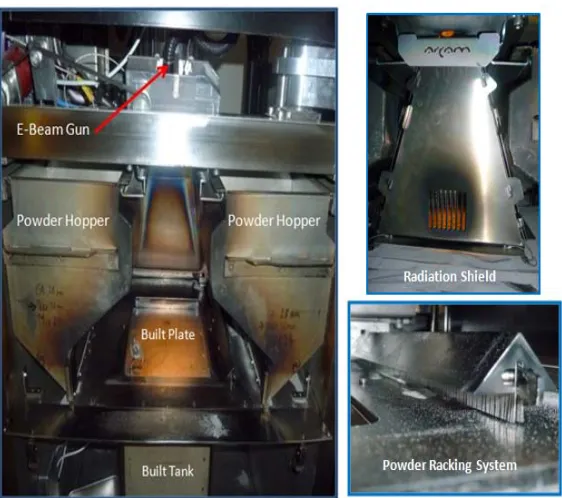
11 in a high vacuum column (5 x 10-4_{mBar). Immediately after electron generation,} the beam is focused and steered by an array of magnetic deflectors, allowing high scan rates of 300 to 5000 cm/sec.

Figure 1.1. EBSM (ARCAM A-2) System Illustration

(34)

12 powder surface, makes the EBSM environment very challenging for in-situ process monitoring.

Additionally, the hard architecture (unable to be modified for in-situ process control) of the ARCAM-AB system common on any production oriented equipment, makes it difficult to modify without affecting the original design, jeopardizing the process stability of the system; reason why the use of modeling and simulation of this additive manufacturing process represents an excellent strategy for material and process evaluation.

1.3. EBSM Process of Ti6Al4V Alloys

(35)

13 machinability required, decreasing the use of low cutting speeds and heavy feed rates [29, 30].

Having a finished or a near finished manufactured part by EBSM process does not imply the required mechanical properties required by the standards for a specific application are met, or how close the EBSM manufactured product is to be use-ready, or if a post-processing procedure is required to modify the resulting material microstructure. Since microstructure and mechanical properties of Ti6Al4V alloys are heat treatment and processing history dependent [17, 31-33], a predictor method is required to estimate the resulting EBSM microstructure, able to mimic the heat evolution originated from a series of melting and re-melting steps occurring every time a new layer of material is deposited [13], making a numerical representation by modeling and simulation to be a rather complex and time-consuming task.

(36)

14 F136-02a and ASTM F1108-04 [34-36], as well as biocompatibility and bioactivity [37, 38].

Early work on aerospace applications showed the advantages of EBSM process on structural metallic components such as rocket engine impellers [33], turbine blades, spare components for environmental control and life support systems (ECLSS) and command and liaison vehicle (CLV) parts[39], among others. On the other hand, aircraft components are currently being manufactured with this technology [40, 41] for quick response tooling, lower recurring unit part costs and faster part delivery times. These improvements come mainly through material requirement changes and design modifications, such as replacing aluminum and steel parts with titanium and making a single part instead of an assembly [27] .

1.4. Modeling the Rapid Prototyping and Manufacturing Process

(37)

15 represents a viable alternative by using fundamental principles in order to study the effect of the process variables over the thermal behavior of the building part.

However, the thermal model for beam-material interaction concerning EBSM becomes rather complex. In particular, the temperature-dependent properties of powder and the consideration of a moving heat source, together with a nontrivial geometry, represent a constraint for analytical solutions of the describing mathematical equations. Thus, numerical methods have been used to calculate the resulting temperature distribution, allowing approximate solutions of three dimensional differential equations with minor losses in accuracy [42]. In particular, the finite-element-method (FEM) subdivides the relevant part geometry into single domains of arbitrary shape which are called finite elements. Thus, the basic functions are only valid within the range of a certain element and comply with the adjacent elements. Consequently, the complete solution consists of a multitude of solutions from neighboring domains.

The Step-Wise Solution

(38)

16 this purpose in mind, many thermomechanical and thermokinetic models have been devised to evaluate residual stress and microstructure, respectively. A practical way to solve a multilayer material deposition or a multidimensional moving boundary problem was initiated with laser-based technologies [43, 44] simulating the laser based deposition process of stainless steel 316L by finite element analysis (FEM) of a traveling volumetric heat source, representing the melt pool in a quasi- steady 2D simulation. The entire built material modeled was discretized in small cubic sub-domains assigning thermal insulation values to the elements (or material) not yet deposited. The movement of the melt pool as the material was deposited was represented by a time and space dependant heating of each element at melting temperature. Once an individual cube or material fraction solution was obtained, it was saved as the initial condition for a new element or material being deposited.

(39)

17 method was later followed by Labudovic and Kovacevic using the same birthing or partial solution events by assigning thermal insulation values to the elements or material not yet deposited through a thermo-mechanical coupled calculation as a representation of a heat source during the deposition of Monel on AISI 1006 [45]; including process parameters such as non-linear physical properties, thermal load, thermal flux densities and latent heat of fusion and neglecting effects such as the convective flow of heat, occurring between the melt pool and the solid part. This evaluation was made using ANSYS software aided by a parametric design language (APDL) for variable definition and simple looping to conduct an iterative analysis until a converged solution for dynamic equilibrium was attained.

(40)

18 again the microstructure evolution caused by thermal cycling was modeled; such model included material thermal properties as well as heat losses by convection and radiation [47-49]. Wang et al., improved this technique by automating the activation and deactivation of the elements in the algorithm model using the a finite element software SYSWELD [50]; program commonly used for heat treatment and welding modeling and compared it with a new approach, named “the dummy material” method, in which instead of deactivating the elements or sub-domains, they were given low conductivity values for energy conservation (in this way the forthcoming element would not be heated). These properties were later updated to the actual thermal conductivity value during element activation representing the material deposition [51].

Despite the accuracy of the previous approaches, the layer-by-layer evaluation required an enormous amount of computing resources, it made necessary the introduction of a fixed boundary method, first introduced by

(41)

19 (1) The thermal conductivity, specific heat capacity, and other materials parameters

in stainless steel 316L powder are temperature-independent; (2) Only heat conduction in build and substrate are considered;

(3) The quasi-steady state is established, i.e. the molten pool does not change size with time;

(4) The temperatures of the element nodes are set as the melting point temperatures;

(5) The part to be formed is adiabatic.

During the modeling and simulation, the activation of elements were performed through a prescribed time step using ABAQUS, linked with the scanning speed of the laser and the amount of mass required to satisfy the melt pool volume. Energy distribution in the laser beam was considered the source of heat, instead of the powder particles at melting temperature. All these approximations were validated by temperature measurements obtained by high speed infrared (IR) thermal imaging during the process and the data was later used to support and correct the simulation values.

(42)

20 temperature as a heat source. This laser energy distribution was later evaluated by

Neela et al. [54], through a multistep transient heat transfer analysis where the heat source was represented as a heat input with a non-uniform Gaussian distribution, where the elements are synchronized by smaller time increments. Herein, a number of elements were activated at each time step and determined by the evaluated volume of melt pool, which depends on the process conditions (powder mass flow rate, powder use efficiency, and scanning velocity).

Finally, the importance of the temperature properties for the powder material was shown by Patil and Yadava [55], where a model for an individual layer is used in metal laser sintering (MLS) to optimize the laser process conditions and avoid thermal distortion during cooling. This was done by the study of a non-uniform transient temperature distribution in the single powder layer of titanium caused by laser irradiation.

1.5. Electron Beam Selective Melting Simulation and Modeling

(43)

21 source analogous to the laser process in terms of melting interaction volume (deep and narrow melt pool). Characterized by smaller beam spot sizes, faster scan rates now possible by the action of magnetic steering systems (contrary to the lower beam steering speeds attained by laser systems) as well as no limitation by reflection attenuation caused by the beam powder material interaction [56].

Besides the use of a different an energy source characterized by a high electron beam power (~4000W), additional process conditions characteristic from the EBSM technology like extremely fast scanning rates (up to 1000 m/s), a vacuum system (5x10-4_{mBar), high cooling rates (~10}○_{C / min) [57], melt pool instabilities during}

the molten state [58-61], together with low alloy element vaporization, powder pushed-away or blown from the build plate caused by static charges accumulation on the powder due to poor contact between the powder particles, preferential grain growth caused by an unidirectional heat flux during the built, thermal stresses from temperature gradients developed during the process and built part porosity caused by un-melted powder particles and inner particle hollow cavities present on the powder feedstock material; makes the electron beam selective melting process modeling and simulation a non trivial task.

(44)

22 composition, specifically metal evaporation. Studies on the evaporation of low alloy elements in Ti6Al4V, due to transient local heating caused by the electron beam on the melt pool, were developed by Powel et al. [62]. Herein, the system was solved using a volumetric solution accounting for the electron beam penetration into the material and a thin film solution evaluating only the temperature distribution below the electron beam. Finally the model was validated by comparing evaporation rates from an electron beam furnace.

(45)

23 Parallel to this work, Zaeh and Kahnert [24],used the concept of reducing the total power during the scan as the temperature attained by the pre-heating stage increases, improving the adhesion between sintered metal layers of H-13 steel; using an adaptive scan strategy as well as developing an adaptive electron beam power input to avoid overheating in areas previously melted. Later, Zäh and

(46)

24 This was followed by Körner and Attar et al. [65] who developed a 2D lattice Boltzmann model (which is an alternative to ordinary computational fluid dynamics models) to study the influence of factors such as the relative powder density, including factors such as the stochastic effect of a randomly packed powder bed, capillary and wetting phenomena on gas atomized (GA) Ti6Al4V powder. The proposed model, although still two dimensional (2D), was able to predict many experimental observations such as the well known surface energy instabilities causing the balling effect. As a result, the effect of the packing density over the melt pool characteristics was observed and a validation process was performed using gas atomized powder as a feedstock material. In this case, results were compared with experimental findings during electron beam selective melting EBSM and the comparison showed to be in good agreement with the simulated results.

1.6. The use of COMSOL Multiphysics Software on Additive Processes

(47)

25 temperature evolution coupled with a moving heat source, not to mention the mutual interdependence on the material’s thermal and physical properties with the temperature. For that purpose, previous researchers have used finite element analysis software packages such as ANSYS, Mathematica and ABAQUS among others, showing the increasing necessity for computer modeling software to improve the qualitative and quantitative process knowledge.

Considering the complexity of the EBSM process involving the conversion of electromagnetic (EM) fields into thermal energy that ultimately melts a metal powder layer. This process contains many variables influencing the outcome of the finished material. Therefore, the selection of a modeling and simulation tool is critical, requiring the use of a powerful system with the ability to be adapted to the very nature associated with electron beam selective melting. This means the coupling of thermal information with phase transformation and finally the as-built material properties.

(48)

inter-26 dependencies with one another. Previous data on similar applications showed the flexibility of COMSOL Multiphysics to model additive processes initially modeling the temperature evolution caused by a laser heat source interaction with a three-dimensional transient heat conductive field on a semi-infinite metallic solid [67, 68].

(49)

27

1.7. Summary

An overall introduction into additive manufacturing and the electron beam selective melting processes was presented; including previous numerical methods used to represent the physical and thermal phenomena taking place during the additive process, with heat sources of high aspect ratio and volume interaction. Finally a review of the strategy used to solve the thermal heat transfer equation on a three dimensional (3D) domain by a moving heat source using a multiphysics solver is described considering its model assumptions and limitations.

(50)

28

2. Materials and Methods

2.1. Ti6Al4V Powder Material

A Ti6Al4V powder was used in this research work with the designation Ti6Al4V (ELI) Grade 23. ELI, stands for extra low interstitial oxygen ~0.13% content with a lower nitrogen carbon and iron composition percentages. This material was obtained from ARCAM-AB and ASM (American Specialty Metals Inc.). The powder material obtained from Arcam-AB was produced by the gas atomization method. This method entails the melting of a metal wire through an array of plasma torches, after which the molten metal is atomized by an argon gas nozzle and cooled at rates between 102_{– 10}3○_{C/sec during precipitation inside an isolated chamber [73, 74].}

Final powder properties can be controlled by adjusting melt temperature and viscosity, alloy composition, metal feed rate, inert gas type, gas pressure, nozzle geometry, gas temperature and residual atmosphere [75].

(51)

29 [76, 77]. The resulting powder is spherical, with a tap density close to 65% of solid substance. Both powders PREP and GA were evaluated in as-received and recycled condition as well as partially sintered, representing the state of the circumventing material during the build and as well as after the additive process.

2.2. Physical Properties Analysis on Ti6Al4V Powders

(52)

30 2.2.1. Particle Morphology Analysis

A Phenon - G2 Pro desktop SEM system was used for the PREP and GA powder morphology study. For this, a monolayer of powder was placed on an aluminum sample holder and graphite tape was used to improve sample conductivity and to promote adhesion with the powder to the tape preventing the particles from flying off once the vacuum system was in operation.

Scanning Electron Microscopy (SEM)

2.2.2. Density and Surface Area

(53)

31

Operation principle

Density by Gas Pycnometry

Gas pycnometry consists of the infusion of helium (He) gas into a porous material contained in a known volume. The gas covers the surface of the sample, obeying the Archimedes principle of fluid displacement. The operating principle corresponds to the gas law PV = nRT. Where P is the gas pressure, V is the volume containing the gas, n is the number of moles of the gas, R is the universal gas constant and T is the temperature of the gas. The equipment used in this analysis was a Ultrapyc 1200e, and the following tests conditions were used:

Table 2.1. He Gas pycnometry measurement conditions

Equipment setup Value

Cell Volume (cm3₎ _149.6553

Analysis Temperature (Celsius) 27.7

Target Pressure psi 10

Type of Gas Helium

Flow Purge (min) 1

Number of Runs Averaged 3

Density by Mercury Pycnometry

(54)

32 Solids by Mercury Intrusion) and consisted of the use of a non-wetting material intruding into the porous sample following the Washburn’s equation [79]. The equation (2.1) dictates that the pressure required for the liquid metal to fill up the pores is inversely proportional to the pore diameter allowing the analysis of particle sizes within the range from 0.003μm to 360μm.

2

cos

4 Dγ

−π θ =πD P (2.1)

Where:

D = 𝑃𝑎𝑟𝑡𝑖𝑐𝑙𝑒𝐷𝑖𝑎𝑚𝑒𝑡𝑒𝑟

𝜋𝐷2 ₌_{𝐶𝑟𝑜𝑠𝑠}_{𝑠𝑒𝑐𝑡𝑖𝑜𝑛𝑎𝑙}_{𝑎𝑟𝑒𝑎}_𝑜𝑓_𝑡ℎ𝑒_{𝑝𝑜𝑟𝑒}_{𝑜𝑝𝑒𝑛𝑖𝑛𝑔}

𝛾 =𝑆𝑢𝑟𝑓𝑎𝑐𝑒𝑇𝑒𝑛𝑠𝑖𝑜𝑛

𝑃 =𝐼𝑛𝑡𝑟𝑢𝑠𝑖𝑜𝑛𝑃𝑟𝑒𝑠𝑠𝑢𝑟𝑒 (𝑢𝑝𝑡𝑜 50 𝑝𝑠𝑖)

And the relation between applied pressure and the minimum pore size into which mercury will be forced to enter is:

4

= − γcosθ D

(55)

33 The system uses a known-volume chamber in which a known sample (powder and sintered material) weight is introduced within the chamber, later pumped down using a vacuum system for sample degassing. After this, the liquid metal (mercury) is introduced to the system until the pressure in the chamber is in equilibrium, and the mercury volume used for pore intrusion is later used to calculate the powder porosity. A low pressure mode 50 psi (345 kPa) was used in this analysis able to attain volumetric resolutions up to 0.1 μL during the mercury intrusion process [80].

Table 2.2. Bulk density measurement setup

Sample and System Properties GA

Powder Powder PREP Sintered GA Sintered PREP Sample Weight (g) 0.7790 0.5093 0.5773 1.1614 Bulk Sample Volume (cc) 0.2990 0.1959 0.2007 0.4354 Total Intruded Volume (cc/g) 0.1509 0.1573 0.1360 0.1373 Hg Surface Tension (erg/cm²) 480.00 480.00 480.00 480.00 Hg Contact Angle 140.00° 140.00° 140.00° 140.00°

(56)

34

Surface Area Measurement by Krypton Adsorption

(57)

35

Sample and system setup

Samples from Ti6Al4V PREP and GA material in powder and partially sintered condition, each with a weight of approximately 14 grams were prepared to be later placed within the sample cell for analysis on a Quadrasorb Si system. The sample powder contained within the analysis cell was degassed for 3 hours at a temperature of 150○_{C and the adsorption time used was 200 seconds.}

2.2.3. Particle Size Distribution by Laser Diffraction

Laser particle analysis is based on the Joseph von Franhoufer model of light diffraction caused by opaque, spherical and non-porous particles. During the evaluation, a specific amount of powder passes through a broadened beam of laser light. This beam is then scattered depending on the particle size traveling in front of it and a particle size distribution is inferred from the angular variation (see

Operation principle

(58)

36 Figure 2.1. Laser diffraction technique (adapted from [84])

Based on franhoufer’s theory, only the size of the particle will affect its diffraction pattern following equation(2.3), where r corresponds to the particle radius, S is the distance from the focal plane and λ is the incident laser wavelength

2 rS

F

π

λ

×=

_(2.3)

Two different sample dispersion methods (wet and dry) were used to estimate the particle size distribution of PREP and GA powders. The laser diffraction

(59)

37 system used for the measurement was a CILAS 1180 for wet analysis, and a Mastersizer 2000 Ver. 5.60 from Malvern Instruments Inc. was used dry evaluation.

The wet mode analysis consisted of the dispersion of 5 grams of Ti6Al4V powder using water as a solvent to ensure the proper particle dispersion, coupled with ultrasound for 60 seconds during the test. Low obscuration values 1.2% (+/- 0.2) was used during the test to guarantee the resolution of small particles, and a total of 5 samples were measured during the analysis.

Figure 2.2. Wet dispersion system Cilas 1800 using a 5gms sample size and obscuration of 1.2%

(60)

38 stream was used to disperse the particles that later were transported through the light detector. Since the instrument operation depends upon obscuration and not the mass of the sample, a total of 158 tests were necessary to use all 250 grams of powder. To analyze each sample, a small amount of powder was placed onto the sampling tray using a vibration feed rate of 75%, and the dispersive air pressure was set at 4 bar. Nitrogen was used as the analysis medium.

(61)

39 2.2.4. 3D Profilometry by Axial Chromatism

Non-contact profilometry has been used to measure the different surfaces involved during the EBSM process, mainly in the case of powder material, where its weak cohesion make it very difficult to measure with conventional contact (stylus) methods. The method used here was 3D optical profilometry using a Nanovea ST400 3D Profilometer. Thanks to its operation principle (axial chromatism), a reliable measurement of rough and non-reflective surfaces is possible without the artifacts and software data manipulation limitations present on light interferometry; offering direct measurements on the surface in focus at higher angles (up to 80○_{) at the same speed as interferometry, and at lower cost.}

The system’s operating principle is based on the refractive index change due to changes in wavelength caused by a diffraction grading. Each wavelength is then used to find a focal point in the surface to generate an image, and the remaining wavelengths (out-of-focus) are canceled during the filtering process. Within the measurement range no height correction must be made and a single monochromatic point is always in focus to construct the image [

(62)

40 Figure 2.4. Axial chromatism operation principle (adapted from [85])

Profilometry measurements were taken with the purpose of correlating the effect of roughness on emissivity values, and to document the EBM processed part surface finish at specific powder size distributions. The surfaces measured included the pressureless sintered powder circumventing the built, the melt (smooth) surface area in line-of-sight of the electron beam and the surface between the solid part built and the surrounding loosely sintered powder.

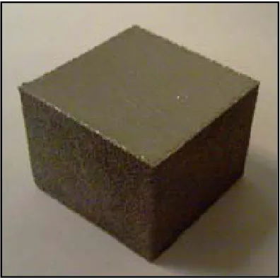
The samples used for this test consisted of an EBSM manufactured solid cube made of Ti6Al4V (1” cube) using PREP powder, where the faces to be measured

(63)

41 were labeled (Face 1 and Face 2). Additionally a partially sintered Ti6Al4V PREP powder sample was prepared with 0.75” in diameter and 0.25” thickness.

Figure 2.5. Image of solid Ti4Al4V (left) and sintered TiAl4V (right) used for 3D roughness analysis

Probe specifications and system measurement setup are specified in Table 2.3 and Table 2.4.

Table 2.3. Probe Specifications 3D Profilometry

Sample _{Ti6Al4V Solid Sintered PREP Powder}

Measurement Range _1100μm _{3.0 mm}

Z resolution (nm) ₂₅ ₇₅

Z Accuracy (nm) ₂₀₀ ₄₀₀

(64)

42

Test conditions:

Table 2.4. 3D Profilometry Test Conditions

Test Specifications Cube Face 1 Cube Face 2 Sintered Powder

Probe (um) 1100 1100 3

Acquisition rate (Hz) 2000 2000 200

Averaging 1 1 1

Measured surface (mm x mm) 27.0 x 27.0 27.0 x 22.0 27.0 x 27.0 Step size (μm x μm) 10 x 15 10 x 15 25 x 50

Scanning Mode Constant speed

2.2.5. Micro Computed Tomography

Computed tomography was initially used as inspection technique on metrology activities for additive manufacturing parts for medical use and is a non-destructive, cost effective and flexible alternative to partial sectioning processes[86]. But, metrology is not the only capability of computed tomography; defect analysis (porosity) has become an area of special interest for this technology. However, the use of this technique for porosity analysis requires the use of an adequate system setup and a higher resolution compared with the currently used for metrology purposes having as a result a new line of products called micro and nano x-ray scanners.

(65)

43 system for imaging) has been previously used, proving to be time consuming and destructive to the inspected sample, allowing flexible technologies like micro computed tomography to occupy its place with optimum results.

Also known as Micro-CT scan; this technique involves a dynamic 2D projection around a single axis of rotation of an object placed on a sample table holder using an X-ray source. The 2D projection is then digitally processed by reconstruction calculations to generate cross-sectional images (see

Operation Principle

Figure 2.6). Finally, 3D CT data is rendered as voxels (volume element) with three-dimensional resolution from a few micrometers.

(66)

44 The X-ray projection principle is based on Beer’s Law (2.4) denoting the x-ray signal reduction as a function of the energy path length and its linear attenuation coefficient,

( )

0

I

=

I

e

−

∫

μ x dx _(2.4)

and considering the effect of the part thickness to be inspected:

0

(

)

I I

=

e

μL

−

_(2.5)

where Iο is the intensity of the incident X-ray beam, I is the X-ray intensity at a

distance L from the source, and μ is the linear attenuation coefficient of the metal measured in cm−1_{. The attenuation coefficient depends on the specific density of the} material, the element atomic number, and the X-Ray beam energy used for the analysis. After the projection data is collected, a comprehensive algorithm is used for 3D reconstruction and final imaging of the object.

Three sample types were used in this analysis; PREP (plasma rotating electrode powder) and GA (gas atomized powder), both in a sintered state and a 1”

(67)

45 square Ti6Al4V cube produced using PREP powder material, as later described in Table 2.5. The equipment used in this analysis consisted of two micro computed tomography systems for defect analysis, consisting on an X-Radia’s (VersaXRM-500) and North Star Imaging (X-View model X-50).

Table 2.5. CT micro scan analysis matrix

Material condition Analysis Equipment used

PREP (sintered) Powder particle inner porosity and _{particle necking} Xradia VersaXRM-500

GA (sintered) Powder particle inner porosity and _{particle necking} Xradia VersaXRM-500

PREP (solid) Porosity analysis Xradia VersaXRM-500

NSI X-View model X-50

Table 2.6. Setup Conditions used on Versa XRM-500

Sample Name PREP (sintered) GA (sintered) PREP (solid)

Source settings (kV/W) 70/6 70/6 150/10

Voxel size (μm) 0.54 0.54 30

Start and end Angle [-180,180] [-180,180] [-180,180]

Number of Views 2000 2000 5000

Time Per View (sec) 5 8 4

(68)

46 Table 2.7. Setup conditions used on NSI X-View model X-50

Equipment Specifications Scan A Scan B

Source Settings: Microfocus X-Ray source (XRayWorX) Microfocus X-Ray source (XRayWorX)

Voltage: 220 kV 205 kV

Current: 93 µA 168 µA

Focal spot size: 20 microns 34 microns

Voxel Size 25 microns 20.4 microns Detector: Varian [1536x1920] Perkin Elmer [2048x2048] _{[XRD 1620/1621 AM/AN]} Pixel pitch: [127 x 127] microns [200 x 200] microns

Framerate: _{(833.333 ms integration time)}1.2 fps

1 fps

(999.911 ms integration time)

Flip: Horizontal Horizontal

Rotation: 270 degree 270 degree

CT Scan:

Type: Step Step

Number of frames averaged: 4 4

Number of projections: 1440 1800

(69)

47

2.3. Thermal Properties of Ti6Al4V Powder and EBSM Processed Parts

Thermal properties for Ti6Al4V material in powder, sintered and solid state were evaluated to be used as a model input for the heat transfer simulation of the EBSM process. Temperature dependence ranges from room temperature to1600 ○_C

were used to measure heat capacity and thermal diffusivity to finally calculate the thermal conductivity of this additive manufacturing material.

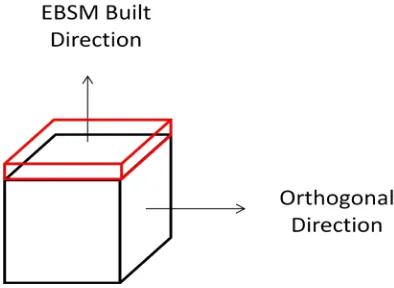
Figure 2.7. Sample orientation illustration used for thermal analysis on Ti6Al4V solid parts

(70)

48 2.3.1. High Temperature Differential Scanning Calorimetry (HT-DSC)

The heat capacity is defined as the quantity of heat necessary to raise the temperature of a system or substance at constant pressure by one degree Celsius. Changes on heat capacity of a metal object of a known mass is measured by the difference of heat flux required to raise the temperature both the sample and a reference material as a function of temperature according to equation (2.6).

Operation Principle

( ) ( )

ref sample base line

p sample p reference

sample ref base line

m DSC T DSC T

C T C T

m DSC T DSC T

−

= × ×

− (2.6)

where Cp corresponds to the heat capacity the sample and the reference material given on (J/g.K) units; m corresponds to the mass in milligrams (mg) for sample

and reference material, and DSC corresponds to the signal obtained from the system corresponding to sample, reference and base line test.

(71)

49 like melting and solid-liquid reactions) the event is considered endothermic; on the contrary when the needed heat flux is lower than the setup value (i.e. in cases like solid-solid transitions and crystallization), the signal present itself as an exothermic occurrence.

Samples used for this test consisted of PREP and GA powder Ti6Al4V material on as-received (never used) and recycled condition as well as solid samples produced by both powder types later processed by EBSM, which characteristics are later described in chapters

Sample and system setup

3 and 4. A 2.5μl volume was used for the powder and sintered material and 20μl for the solid samples. Solid PREP and GA Ti6Al4V disks were machined to fit 5mm in diameter and 1mm thickness and both type of samples were contained on a platinum (Pt/Rh, 30μl volume) crucible holder.

Specific heat capacity was measured using a power compensated DSC 404 -F1 Pegasus_-_{differential scanning calorimeter from NETZSCH instruments.}

(72)

50 occur. In this way the heat flow is measured in a more direct manner compared to conventional DSC were the heat capacity measurement is obtained indirectly from temperature differences between sample and reference materials as previously described in equation(2.6).

Additionally, the system was equipped with a platinum-rhodium furnace capable of operation from -150°C to 1650°C and is vacuum-tight, so samples could be tested under purely inert, reducing, or oxidizing atmospheres, as well as under vacuum. Instrument control and data acquisition are accomplished via a 32-Bit MS -Windows_Proteus_{software and electronics system.}

(73)

51

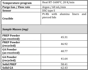
Table 2.8. Differential Scanning Calorimetry measurement setup using DSC 404 F1Pegasus®

Temperature program Heat RT-1600°C, 20 K/min Purge Gas / Flow rate Argon / 60 mL/min

Sensor DSC type S

Crucible

Pt-Rh with alumina liners and pierced lids

Sample Masses (mg)

PREP Powder

(as-received) 45.31

PREP Powder

(recycled) 46.92

GA Powder

(as-received) 40.77

GA Powder

(recycled) 41.64

Solid PREP 58.41

Solid GA 62.43

2.3.3. Laser Flash Analysis (LFA)

Laser flash is a thermo analytical method, consisting on the heating of a disc-shaped sample on one of its sides using a laser pulse and measuring the increase in temperature caused by the absorbed energy on the opposite surface (see

(74)

52 surface of the sample. Thus, the resulting rear-face temperature rise is recorded and analyzed to calculate the thermal diffusivity of the material whether it is in powder, sintered, or solid form[87].

Figure 2.8. Laser flash operation principle

The thermal diffusivity α indicates the material’s ability for heat propagation by conduction when the temperature change with time (transient process); this property is measured by the ratio between the sample area L2_{and the half-time}

(t1/2) required for a laser pulse created by the laser flash system to increase the sample temperature from the baseline to an specific analysis temperature. This

(75)

53 property has a dimension of area over time expressed in m2_{/s as seen in} equation(2.7).

2 1/ 2

0.13879 /L t

α = _(2.7)

Figure 2.9. Half time temperature pulse calculation

Thermal conductivity is the quantity of heat transmitted as a result of a temperature gradient with a direction normal to the surface and is calculated by,

(76)

54

Cp

λ α

=

ρ

_(2.8)

where λ is the thermal conductivity, α is the thermal diffusivity, Cp the sample heat

capacity, and ρ the sample density.

An LFA 427 system was used to calculate the thermal diffusivity based on the thermal laser flash method conducted according to standard test ASTM E 1461-11. Two type of samples with replicas (n=2) from PREP and GA Ti6Al4V as-received powder, and EBSM processed solid condition, were prepared for this test with 12.7 mm diameter size and 2 mm thickness. The system heat source for diffusivity measurements was set with a laser pulse power of 2.1kV and a pulse width of 0.5 µs.

Sample and system setup

2.3.4. Remote Infrared Temperature Measurement (IR)

(77)

55 Remote temperature measurement is possible through the detection of infrared energy emitted from all objects at temperatures above the absolute zero energy (0○_{K). This radiated energy is later converted into a thermal image of the}

object being surveyed [ Operation principle

88].

The temperature system used here consisted of a FLIR SC5600-M camera using a Indium antimonide InSb photovoltaic sensor, operating on the 2.5 - 5.1 micron waveband range. Since the measurement range for the emissivity evaluation exceeds the 300○_{C, neutral density germanium filter (0.3 O.D with 25mm diameter),}

spectrally flat between 2-14 microns, was used inside of the camera to attenuate the signal enabling the temperature reading up to 1000 ○_C.

System setup

2.3.5. Fourier Transform Infrared Analysis (FT-IR)

(78)

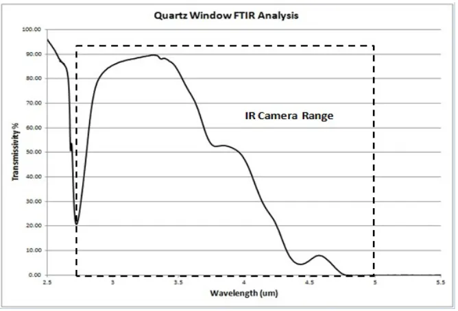
56 suitable view port transparent in the infrared study range was necessary. Thus a quartz window was chosen in terms of availability and its infrared trasmissivity was measured using the FT-IR technique. Furthermore the data obtained was later used to calibrate the remote temperature setup.

Figure 2.10. Nicolet 8700 FT-IR System

(79)

57 2.3.6. Emissivity measurement

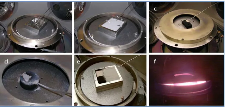
A vacuum system was used to mimic the low pressure environment present inside of the EBSM chamber during the build. A graphite heater was used to heat the samples up to 800○_{C (}

System setup for Ti6Al4V emissivity calculation

Figure 2.12.f), since common built temperatures used on Ti6Al4V are in the range of 625 to 700○_{C [17].}

(80)

58 The vacuum system was equipped with a quartz viewport, through which the infrared camera could view the test sample. The standard deviation of the temperature measurement from the FLIR SC5600 infrared camera is approximately 1○_{C within the range of analysis.}

EBSM solid parts made out of PREP and GA powder were sectioned and its surfaces (smooth surface caused by the e-beam melting and rough surface created by the contact with the circumventing powder during the built Figure 2.12. c through e) were partially coated with graphite to serve as a black body radiation reference point.

Figure 2.12. Emissivity sample setup: a. EBSM processed Ti6Al4V holder; b. Ti6Al4V powder; c. Solid Ti6Al4V partially coated with graphite; d. Sintered Ti6Al4V powder; e. Powder and partially graphite coated rough Ti6Al4V solid; f. Side view image

(81)

59 An EBSM solid block (manufactured using Ti6Al4V PREP powder material) was properly machined to fit the samples and ensure a uniform heating surface while containing the powder material (see Figure 2.12a. and b). A quartz window was chosen for its vacuum compatibility and spectral concordance to the camera range and operating temperature[88]. Additional calibration was required on the viewport window used to remotely measure the temperature, since a flat IR transmissivity in the range of 0.1 – 3 microns in wavelength was necessary. It was found the window was not entirely transmissive to infrared radiation (see Figure 2.13) within the evaluation range and further calibration was necessary using a black body (BB) radiation correction protocol.

(82)

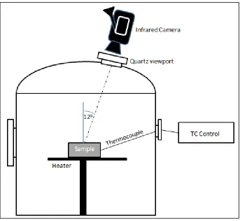
60 Figure 2.14. Viewport correction setup

The view port spectral calibration consisted on the infrared temperature measurement of parts coated with graphite (for maximum emissivity results) with and without using the view port (see Figure 2.14) to create a correction curve as previously described by Xu and Fisher [89] and depicted in Figure 2.15. Data was obtained from room temperature up to 300○_{C and a linear polynomial solution}

(83)

61 Figure 2.15 Thermal Camera Calibration with black body source behind Quartz

window

Figure 2.15 shows the calibration result with a blackbody (BB) source behind the quartz window. The temperature reading from the camera is linear with the actual temperature, and this characteristic has been verified with different surfaces both in air and in high vacuum environments. Once the calibration was performed, the data provided by the IR camera was corrected and the emissivity values were estimated as seen in section 4.4.

T(IR) = (0.324*Thermocouple) - 23.601 R² = 1

0 50 100 150 200 250 300 350

0 200 400 600 800 1000

Te mp era tu re fro m I R C ame ra οC

Temperature from Thermocouple ο_C

Temperature Correction Data