Transactions of the 17th International Conference on
Structural Mechanics in Reactor Technology (SMiRT 17) Prague, Czech Republic, August 17 –22, 2003
Paper # B02-4
Topology Optimization of the Structure with Material Properties Changing
Ryszard Kutyłowski
Institute of Civil Engineering, I-14, Wrocław University of Technology, Wrocław, Poland
ABSTRACT
The problem of changing the material properties during the working time of the nuclear reactor structures is considered. When the temperature is growing up in some parts of the structure the material properties are changing which means the value of the Young’s modulus is decreasing. The main problem discussed in this paper is to analyse and to compare the topology of the structure before the decreasing of the Young’s modulus with the topology of the structure after decreasing. We can find an answer on the question how to design the structure, to avoid the problems when in some parts of the structure, because of the material properties changing, the material is not able to carry the load. Proposed algorithm let to analyse the structure and show a new distribution of the material.
During the design process the designer should identify the weak regions of the structure which may be destroyed as the first during an accident. This paper gives the tool which may be useful for safe design of the structure.
We consider the variation formulation of the optimization problem. The objective is defined as the total strain energy, which is an equivalent to the mean compliance of the structure. The objective is minimizing under the constraint put on the mass of the structure, which is equal or less to the available mass. The available mass is assumed as a constant value for considered structure during the optimization process. What is important, the algorithm is working for the fixed design domain. The artificial approach, which is used here, leads to the material – void distribution of the material. Original, very effective topology optimization algorithm is used here. It let us to obtain the optimal topology within very small optimization steps number.
To numerical realization of the problem the finite element method is used, as the best method if we compare the real structure and the numerical model. Some examples are presented to show the optimal topology changes after changing the material properties in some parts of the structure.
KEY WORDS: Topology optimization, the mean compliance, the artificial approach, material-void distribution, changing the material properties, optimal topology for destroying structure.
INTRODUCTION
Considered problem is the base problem for the case for the abnormal situations, which can be happened during the working time of various structures. As an example let us realize that the temperature in some parts of the structure (of the reactor covers structure for example) is growing up. It may happen because of an accident with the nuclear fuel or because of any other reasons including unexpected events (for example explosion). The structure should work as long as possible in this case and when the structure will not be able to carry the load, it should collapse as safely as possible. This means that collapsing process should be foreseeable and should proceed in earlier designed manner.
The designer should to design the structure as an optimal one. This means, that the structure should be optimal structure during normal working time and during abnormal situations should be as optimal as it is possible.
a) b)
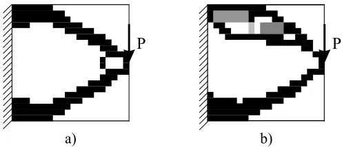
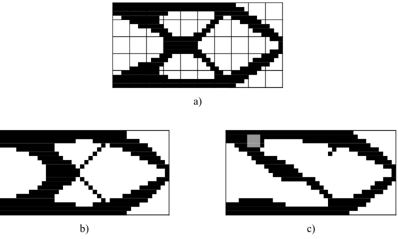
Considered problem refers to one kind of continuum material placed within the design domain. When the material properties in some design domain regions are changing we have one base material and as many additional materials as many regions with changed material properties there are within the design domain. This discussed material property will be the Young’s modulus. In the Fig. 1 we have the optimal topology for the well known in literature benchmark (Fig. 1a) and in the Fig. 1b we have the same topology with marked some destroyed regions (the Young’s modulus was decreased). Various shades of grey mean various value of the Young’s modulus. The problem is how to relocate the mass within the design domain to obtain the optimal topology of the structure. We can sometimes predict where the destroyed areas may come into existing. This let us to solve the optimization problem for the design domain with some regions with various weaker materials. For example it may be the case, shown in the Fig. 1b, where the regions with the shades of grey are fixed and the available mass should be distributed taking into account these “grey” regions. When we will obtain the optimal topology for this case we should take the base optimal topology (Fig. 1a) and we should find the common shapes. Additionally, the design process let us obtain new optimal topology which fulfill the optimality criteria for normal and abnormal situations.
During unexpected events the changing process of the Young’s modulus may be linear or even nonlinear. Sometimes after very fast changing process it may be constant. We should test how changes the topology for mentioned Young’s modulus changing. The changes of the Young’s modulus may be different in various domain regions and this will be taken into consideration in optimization process.
Finally we will be able to obtain the optimal topology for normal and abnormal situations.
The second way of designing of the structure may be as follow: proposed approach may be applied to design a smart structure – defined here as a structure which shape may be changed during the collapsed process. This deals with special civil engineering structures or mechanical structures, which have special sensors system. In case of unexpected event the information of this event is detecting by sensors system and next is analysing by the analysis and decision system. The optimization algorithm shows a new optimal topology and finally the actuators modify the mass distribution according to the destroyed regions.
THEORETICAL BASIS
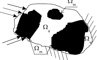
The variation, boundary problem is stated. The design domain Ω is initially random fulfils by the material in m
Ω subdomain and by void in Ωm subdomain (Fig. 2).
The topology optimization problem presented in this paper is based on [1] where it is formulated for a continuum structure. This general approach is in agreement with well known formulation of the topology optimization problem [2]. We have to answer the question where within the design domain the mass has to added or to be taken away. The first step is the homogenization the available mass within the whole design domain. Solving the boundary problem we can obtain the solution of it, finding the unique vector of the displacement. The mean compliance of the structure, defined below, is the reciprocal to the stiffness of the structure:
( )
∫
∫
Ω ∂Ω
+ Ω =
Π
t
ds v t d v b x v
x i i i i
E , ρ( ) (1)
Fig. 2 Initially, random material distribution
Ω m
Ω v
Ωm
where ρ(x)bi is the component of the body forces , vi is the component of the displacement field and ti is the component of the traction force. The objective is defined as the total strain energy which is an equivalent to the mean compliance of the structure:
( )
x,v 2 I(x,v)E Π
Π = (2)
where
Ω ρ
Π
Ω
d v e v e x v x C v
x ijkl ij kl
I( , ) ( , , ( )) ( ) ( )
2 =
∫
(3)The available mass is defined as:
1 0 ,
0=αm <α<
m (4)
where
ρ
V
m= (5)
and α is the mass reduction coefficient, which is assumed separately for each optimization process. Since parameter α is less than one, ultimately we shall obtain a structure which will not occupy the whole design domain with density ρ. The volume V is the volume of the design domain Ω. The optimization process is constrained by:
0 1 )
(
0
= − =
m m
H ρj j (6)
which means: the mass of the structure in the j-step of optimization is less than or equal to the available mass. The objective can be stated now as:
) (
)) ( ( )
), (
( x C x e e d d m0
F =
∫
iklm ik lm +∫
h −Ω Ω
Ω ρ λ Ω ρ
λ
ρ (7)
where ρh is the density of homogenized material and λ is the Lagrangre multiplier. Elasticity tensor Cijkl is a function of Young’s modulus:
))) ( ( (E x C
Cijkl = ijkl ρ (8)
For updating Young’s modulus in the j-step during the process the following artificial density function is used:
3 0
1( ) ( )
h j j
j E
E
ρ ρ ρ =
+ (9)
where Ej+1 is Young’s modulus of each design point for the j+1 step, E0 is an initial Young’s modulus, and
j
ρ is an “artificial” density of each design point for the j step. The above definition is based on the Bendsoe [3] and Ramm [4] formulations proposed in general, the Young’s modulus dependence of the density of considered design point. The wide spread analysis of various updating definitions was made in [5], where it was shown the most effective definition written in Eq. (9).
of grey in the Fig. 1. Cdiklm and Cviklm are the elasticity tensors of mentioned above regions respectively, and m
l k i
C is the elasticity tensor for material with the density ρ. In the above equation each considered region may consists of many separate subdomains.
(
)
(
)
(
)
− + − + + − + + + + + =∫
∫
∫
∫
∫
∫
d d v v m m v d m m d x m d x m d x d e e x C d e e x C d e e x C x x x F d d v v m m v m l k i m l k i v d m l k i m l k i d m m l k i m l k i d v m Ω Ω Ω Ω Ω Ω Ω Ω Ω Ω γ λ Ω η λ Ω ρ λ Ω η Ω γ Ω ρ λ λ λ η γ ρ _ 0 _ 0 _ 0 ) ( ) ( ) ) ( ) ( ) ( ) ( ) , , ), ( ), ( ), ( ( (10)Searching for the stationary point of the above functional, we obtain the equations which describe considered problem. Because of completing the objective by some additional terms, minimazing the objective following additional equations are obtained:
(
)
(
)
d d m d x F e e x C F d d d m l k i m l k i d Ω Ω Ω γ λ λ γ γ γ _ 0 ) ( 0 , 0 ) ( 0∫
= ⇒ = ∂ ∂ = + ∂ ∂ ⇒ = ∂ ∂ (11)The mass of Ωd regions fulfil the equation:
d
v m
m m
m0 = 0_Ωm + 0_Ω + 0_Ω (12)
The total sum of the mass of the structure is constant and is a sum of the mass in all regions within the design domain Ωm, Ωv,Ωd .
EXAMPLES
Presented in the above section theory was formulated for the continuum structure within the design domain. We can treat continuum structure as a finite set of the material point parametrized by the geometrical coordinates and by mechanical properties of the point material. The geometrical size of the material point are enough small to treat all of them together as continuum structure. The material point during the optimization process becomes the design point. Because even in theoretical consideration the continuum structure is discretized into the material points, it seems, the finite element method is the best numerical method for numerical realization of the problem. In this case there is the mutual correspondence between the real structure and its theoretical model from one hand and the mutual correspondence between the theoretical model and FEM model from the second hand.
We will find the optimal topology for constant, lower value of the Young’s modulus and for decreasing during the process value of the Young’s modulus.
The following threshold functions are used to obtain optimal topology:
α α
j TF
j TF
0125 . 0
1 . 0
2 1
= =
(13)
where j is the step number and α is the mass reduction coefficient. Most of the pictures were obtained using
1
TF . Those which were obtained using TF2 have this information enclosed in the text. α coefficient is assumed as
equal 0.3 in the most of figures except Fig. 7 where it is assumed as equal to 0.5.
The first example is shown in the Fig. 3 where on the left side we have the base topology shown in the Fig. 1a. In the middle we have the topology for the Young’s modulus decreasing during the process follow the function
j E
E= 0 . In the Fig. 3c the differences between Fig. 3a and 3b are shown. During decreasing of the Young’s
modulus the mass was taken away from these elements which are marked by “x” letter placed on the grey field. To some elements the mass was added (they are marked by darker shade of grey with the letter “a”). Analizing this picture we can see which elements are the base elements (did not be destroy). Additionally we can make these base elements stronger to be able to carry the load even during the accident. In this example the step number of the optimal, zero – one topology was equal fourteen, which means the Young’s modulus was decreased maximally fourteen times within all the structure.
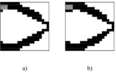
Some elements of the structure may be destroyed faster (for example the temperature in some regions may be higher than in others). In the Fig. 4 in marked by the shade of grey region, additionally the Young’s modulus is lower thousand times than in other elements. This means that these regions do not be able to carry the load. In the Fig. 4a we can see that algorithm can not to take away the mass from two elements, in which it is written “m”. This means using TF1 we can not obtain the optimal topology. Let us to try to use TF2. The optimal topology is shown
in the Fig. 4b. The weaker region is surrounded by material.
x x a
x x x x a a
x a
x x
x x x x x x
x a
x x x x a a
x x a
a
a) b) c)
Fig. 3 Base example topologies
a) b)
It is interesting how the algorithm works when besides decreasing the Young’s modulus of all the structure, additionally, for example in upper left part of the structure, the Young’s modulus will be lower ten or thousand times in nine elements, what is marked by the shade of grey in the Fig. 5b. Unfortunately when the Young’s modulus is lower ten times (the difference is not high), in the Fig. 5a we have the topology where algorithm left material within three upper elements (it is marked by very light shade of grey ). These three elements do not work on the right side where we have the Young’s modulus lower thousand times. In this case we can see a new one topology. The algorithm creates the support below the weaker region.
Analyzing the Fig.4 and Fig.5 it is clear that the size of additional weaker material is the cause of the changing the optimal topology.
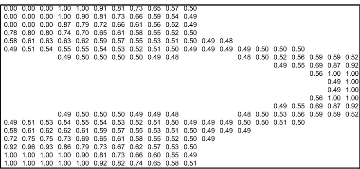
When we have the same example, as in the Fig. 5, but the Young’s modulus decreasing with j2 instead with j we can not obtain the optimal topologies. This means the decreasing process is too fast and there is no exist the optimal topology in this case. In the Fig. 6 there is the topology in number mode for the Young’s modulus in upper region lower 1000 times. There is the distribution with the densities in the range from 1 to about 0.5 (except weaker region of nine elements). In the next step after presented, the problem diverges.
In the Fig. 7 the longer cantilever beam is shown. It is divided into 20 x 40 elements. The mass reduction coefficient α is equal to 0.5. The base topology obtained using TF1is shown in the Fig. 7a. When the Young’s modulus decreases linearly according to the number of optimization steps TF1 it do not let us to obtain optimal
topology. We need weaker threshold function. As in previous examples, we can use TF2. The optimal topology is shown in the Fig. 7b, where more mass was moved from the right cross part to the left direction. Right cross part is very weak, and additionally material was moved to up and down parts of the beam. This means, the inside cross is
Fig. 6 Topology in number mode
0.00 0.00 0.00 1.00 1.00 0.91 0.81 0.73 0.65 0.57 0.50 0.00 0.00 0.00 1.00 0.90 0.81 0.73 0.66 0.59 0.54 0.49 0.00 0.00 0.00 0.87 0.79 0.72 0.66 0.61 0.56 0.52 0.49 0.78 0.80 0.80 0.74 0.70 0.65 0.61 0.58 0.55 0.52 0.50
0.58 0.61 0.63 0.63 0.62 0.59 0.57 0.55 0.53 0.51 0.50 0.49 0.48
0.49 0.51 0.54 0.55 0.55 0.54 0.53 0.52 0.51 0.50 0.49 0.49 0.49 0.49 0.50 0.50 0.50
0.49 0.50 0.50 0.50 0.50 0.49 0.48 0.48 0.50 0.52 0.56 0.59 0.59 0.52 0.49 0.55 0.69 0.87 0.92 0.56 1.00 1.00 0.49 1.00 0.49 1.00 0.56 1.00 1.00 0.49 0.55 0.69 0.87 0.92 0.49 0.50 0.50 0.50 0.49 0.49 0.48 0.48 0.50 0.53 0.56 0.59 0.59 0.52 0.49 0.51 0.53 0.54 0.55 0.54 0.53 0.52 0.51 0.50 0.49 0.49 0.49 0.50 0.50 0.51 0.50
0.58 0.61 0.62 0.62 0.61 0.59 0.57 0.55 0.53 0.51 0.50 0.49 0.49 0.49 0.72 0.75 0.75 0.73 0.69 0.65 0.61 0.58 0.55 0.52 0.50 0.49
0.92 0.96 0.93 0.86 0.79 0.73 0.67 0.62 0.57 0.53 0.50 1.00 1.00 1.00 1.00 0.90 0.81 0.73 0.66 0.60 0.55 0.49 1.00 1.00 1.00 1.00 1.00 0.92 0.82 0.74 0.65 0.58 0.51
a) b)
less important when the material is becoming weaker. As in the previous examples we want to analyse the situation when in some parts of the structure (marked by the shade of grey), the Young’s modulus decreases additionally. It is less than thousand times in comparing with the base structural material. This means the structure in this region is completely destroyed. The algorithm construct the optimal topology by another way, surrounded the weak region and created transverse connection from the left top to the right down part of the beam.
Next we try to analyze the structure for which we have two additionally decreased regions, besides the decreasing the Young’ modulus of all the structure. In the Fig. 8a the optimal topology for the base material without decreasing the Young’s modulus with two regions of the Young’s modulus less ten times than in the base material is shown. The same example without these two regions there is in the Fig. 3a. In the Fig. 8b the Young’s modulus is decreasing linearly with the optimization step number. The optimal topology a little bit changes, but the material can not surrounds the weaker material. Because the lower left part of the structure has more material it is possible that such structure is able to carry the load. In the Fig. 8c marked material has the Young’s modulus one thousand weaker than the base material. Probably such big difference between material characteristics is a cause of surrounding these weak regions by the base material, which is becoming weaker too. The optimal shape in general in all the pictures in the Fig. 8 is similar and may be a base for optimal designing the structure in case if material may be destroyed in marked regions, which are in the places, where in the Fig. 3a we have the material.
a)
b) c)
Fig. 7 Topologies for 20 x 40 beam and = 0.5α
a) b) c)
lower ten times and in the second (right, down one) it is lower one thousand times. This is marked in the Fig. 9 by various shades of grey. Lighter shade of grey means weaker material. Unfortunately in the left picture material does not surround the weaker region, but as it was mentioned earlier this (E = 0.1 E0) can cooperate with the base material. From the other hand it is more safety when the base material surrounds the weaker one. In the Fig. 9b there is the topology for TF2. Choosing longer, but more precise optimization path we can obtain the topology which
satisfy us. Obtained shape is optimal and we can observe the good agreement with designer intuition. From the other hand the designer should to check if obtained optimal topology is able to carry the load (the strength of material conditions and deflection conditions should be satisfied).
When, for the same as in the Fig. 9b example the decreasing function is changing from dividing by j (the number of the optimization step) into dividing by j2 we can not obtain the optimal topology (Fig. 9c). The material is too weak and it is not able to work longer. Some material was placed below the weaker region and it has no any connection with the structure, what is dangerous and in lower part between horizontal lower part and diagonal part it may come into existance a joint, what is dangerous too.
SUMMARY AND CONCLUSIONS
The problem of topology optimization of continuum structure made of materials which material properties are changing during the real, structures working time was solved. The optimal topology changes when material properties changes and the topology depends on:
1. the size of the region within which there are the changes, 2. the number of regions with changes,
3. the value of changed material properties.
The designer should analyse many topologies to find common elements, which should be as strong as possible. Taking into account various solutions for various decreasing the Young’s modulus models we can find the hints for designers how to design the structure for working in normal and abnormal situations (including the accidents).
Additionally presented algorithm may be useful in macro and micro scale, when in some parts of the nuclear power plant structures we have some elements which should be designed as a smart structures.
REFERENCES
1. Kutyłowski R., “On an effective topology procedure”, Structural and Multidisciplinary Optimization, Vol. 20, 2000, pp. 49-56.
2.Bendsoe M. P., Optimization of Structural Topology, Shape and Material, Springer Verlag, Berlin, Heidelberg, New York, 1995.
3. Bendsoe M. P., “Optimal shape design as a material distribution problem”, Structural Optimization, Vol. 1, 1989, pp. 193-202.
4. Ramm E., Bletzinger K.-U., Reitinger R. and Maute K., “The challenge of structural optimization”. In: Topping, B.H.V.; Papadrakakis, M. (eds.) Advances in Structural Optimization, (Proc. Int. Conf. on Computational Structures Technology, held in Athens), Edinburgh: Civil Comp Press, 1994, pp. 27-52.
5. Kutyłowski R., “About the artificial approach in topology optimization in meaning of the convergence problem”.
Z. Angew. Math. u Mech, Vol. 80, Suppl.2, 2000, pp. S535-S536.
a) b)
Fig. 9 Topologies with additional two various weaker regions