The Joint Replenishment Problem and Extensions.

(1)

ABSTRACT

LIN, YU LIANG. The Joint Replenishment Problem and Extensions. (Under the direction of Dr. Shu-Cherng Fang).

The Joint Replenishment Problem (JRP) is to determine the lot sizes and replenish-ment cycle time of a group of items in a single facility inventory system over an infinite planning horizon. In this dissertation, we focus on modeling and proposing algorithms of two extensions of the JRP.

The first study investigates the JRP under cycle time constraints that are popular in practical inventory systems. The constraints can also be extended to restrictions such as minimum order quantity, delivery frequency, and storage capacity limitations. Based on our theoretical analysis on the optimality solution structures, we categorize the items into four types and develope an efficient algorithm for solving this constrained JRP. The numerical experiments show that our proposed algorithm is effective by comparing with the existing approaches in the literature.

The second study investigates a logistics plan that integrates inventory control and districting problems. When many customers scattered in a wide area, it may require us to solve a districting problem which divides them into some mutually exclusive zones. Then, customers in the same zone would order the same group of items jointly from a single supplier, which corresponds to a multi-customer joint replenishment problem (MJRP). The objective of this study is to solve the integrated problem called multi-customer joint replenishment problem with districting consideration (MJRPDC).

(2)

real-life example for a bank company indicates that the proposed method is effective for solving MJRPDC with an average run-time growing in a quadratic rate of the number of customers. Moreover, a sensitivity analysis is conducted to provide the decision-makers with some managerial insights and strategic implications.

(3)

(4)

The Joint Replenishment Problem and Extensions

by Yu Liang Lin

A dissertation submitted to the Graduate Faculty of North Carolina State University

in partial fulfillment of the requirements for the Degree of

Doctor of Philosophy

Industrial Engineering

Raleigh, North Carolina 2019

APPROVED BY:

Dr. Michael Kay Dr. Ming-Jong Yao

External Member

Dr. Russell King Dr. Yunan Liu

(5)

DEDICATION

(6)

BIOGRAPHY

(7)

ACKNOWLEDGEMENTS

First, I sincerely appreciate my advisor Prof. Fang and Prof. Yao for their valuable guid-ance and support throughout my Ph.D. study. They are the best teachers and mentors I have ever met, and they have a significant impact on my life. I would also like to thank Prof. Lin for his instruction and experience sharing during my graduate study. I am so lucky to be exposed to different disciplines, each showing a unique attitude toward education and life.

I am also very grateful to my committee members - Prof. King, Prof. Liu and Prof. Kay for their valuable comments and suggestions for my research and presentations. Their encouragement inspired me to excel in my work and be more confident.

Also, it is a blessing for me to have so many wonderful friends who share a happy but tough school life. To my friends at NC State: Qi, Shan, Kiwy, James, Zheming, Fengming, Sha, Tiantian, Yang, Ling, Xiaohu, Ziteng, Peihua, Daniel and Jessie; my friends at NCTU: Iris, Yu-Che, Chia-Jun, Liam, and Andy; and my friends in Raleigh: Lin’s family, the Smith’s family, the Leanhardt’s family, Karla, and so many others that I cannot list them all. I’ll never forget your willingness to help me, to encourage me, to believe in my ability to achieve my dreams.

(8)

LIST OF TABLES

Table 2.1 Solution approaches for deterministic demand models . . . 23

Table 3.1 The parameters in the demonstrative example . . . 70

Table 3.2 The search process of the demonstrative example . . . 72

Table 3.3 Type change in the search process . . . 74

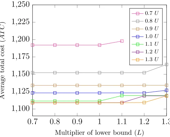
Table 3.4 The impact of upper bounds and lower bounds on the average total cost . . . 74

Table 3.5 The experimental settings in [77] . . . 76

Table 3.6 The search process of the example in [77] . . . 77

Table 3.7 The experimental settings in [43] . . . 78

Table 3.8 The search process for the example in [43] . . . 79

Table 3.9 Average total cost savings from the PD algorithm whenn= 20 (%) 83 Table 3.10 Calculation time savings from the PD algorithm when n= 20 (%) 84 Table 4.1 The binary string corresponding to the coordinates of three zone centers . . . 114

Table 4.2 The districting results of the 80-branch example with 5 zones . . . 120

Table 4.3 The total costs under different α and p. . . 121

Table 4.4 The total costs under different Md and p . . . 123

Table 4.5 The run-time w.r.t. the number of customers . . . 125

Table 4.6 The average run-time with and withoutβ2 . . . 127

Table 4.7 The run-time w.r.t. the number of items . . . 128

Table 4.8 The run-time w.r.t. the number of customers . . . 132

(11)

LIST OF FIGURES

Figure 1.0.1 Three levels of supply chain management decisions . . . 2

Figure 1.1.1 Behavior of inventory level with time in EOQ model . . . 4

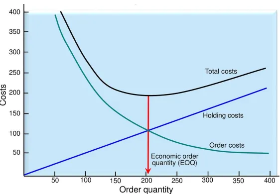
Figure 1.1.2 Graphical representation of the economic order quantity . . . 5

Figure 1.1.3 An example of joint replenishment . . . 6

Figure 1.1.4 Behavior of inventory in joint replenishment . . . 7

Figure 2.2.1 The AT CP oT(ki(B), B) cost function . . . 24

Figure 2.2.2 The AT CP oT(B) cost function . . . 25

Figure 2.3.1 The scenario in [12] with predetermined routes . . . 32

Figure 2.4.1 The framework of GA . . . 40

Figure 3.3.1 Optimal Multipliers in Four Types . . . 54

Figure 3.3.2 Type Changes . . . 63

Figure 3.4.1 The impact of upper bounds and lower bounds on the average total cost . . . 75

Figure 3.4.2 Percentage savings from the independent order . . . 84

Figure 3.4.3 Calculation Time Comparison . . . 85

Figure 3.4.4 Number of intervals Comparison . . . 86

Figure 4.1.1 The scenario in [12] with predetermined routes . . . 89

Figure 4.2.1 Two districting examples with 10 customers and 3 zones . . . 93

Figure 4.2.2 The cycle times in an example with 3 zones and 10 customers . . 94

Figure 4.4.1 The framework of the proposed solution approach based on GA . 111 Figure 4.4.2 Three grid points stand for the centers of three zones . . . 113

Figure 4.5.1 The districting results of the 80-branch example with 5 zones . . . 120

Figure 4.5.2 The average run-time grows in a quadratic order w.r.t. no. of cus-tomers . . . 126

Figure 4.5.3 The average run time grows in a quadratic order w.r.t. no. of items 129 Figure 4.6.1 The framework of the heuristic method . . . 131

Figure .2.1 Random experiments results (I) . . . 154

Figure .2.2 Random experiments results (II) . . . 155

Figure .2.3 Random experiments results (III) . . . 156

(12)

Chapter 1 Introduction

Supply chain management (SCM) involves a series of key activities and processes that must be completed by several parties such as suppliers, producers, distributors, retailers, and customers. The SCM activities including forecasting, production, warehousing, in-ventory management, procurement, and transportation. Those activities coordinate the flow of materials, information, and money concerned directly or indirectly by all par-ties. The primary goal of SCM is to collaborate with channel partners and perform the functions efficiently and profitably.

(13)

oper-Figure 1.0.1: Three levels of supply chain management decisions

Source: https://www.hoeveler-holzmann.com/en/services/supply-chain-management/

ation level decisions are related to day-to-day processes such as logistics planning and production scheduling.

(14)

1.1 Motivation

It is well-known that supply chain management is critical for suppliers, manufacturers, and consumers. According to the [102], the value of current business inventories in the United States is more than $1.9 trillion. For many companies, inventory is the most sub-stantial asset balance owned by the company because they have to ensure the continuity of supply and fulfill customer’s demands. If the amount of cash tied up in the inventory balance can be reduced, then the companies are more flexible to utilize their assets and improve efficiency.

The lot-sizing inventory has been very extensively adopted in the production and distribution systems. It takes advantages whenever quantity price discounts, shipping costs, setup costs, or similar considerations make it more economical to purchase in larger lots than needed. The lot size inventory is differentiated from inventory that is purely demand driven. The decision makers need to coordinate the lot sizing of batches (or, equivalently, the replenishment cycle time) of items to balance inventory holding costs and the fixed costs associated with orders. If the executive managers may effectively apply the concept in their production/inventory systems, they could manage to meet customers’ demand satisfactorily and importantly, to reduce significant cost. Therefore, the lot-sizing problems are of great interests to the researchers in theory and practice.

(15)

Figure 1.1.1: Behavior of inventory level with time in EOQ model

reorder quantity such that the total costs of inventory including fixed cost and holding costs are minimized as depicted in Figure 1.1.2.

The EOQ model can be a valuable tool for decision makers. However, the simplicity restricts the applications in practice. For example, if we would order multiple products from a single supplier, and each product is ordered according to their EOQ policies, then it may create so many cycle time patterns and cause operational difficulties for the suppliers. Another restriction of EOQ takes place when the fixed cost is not charged separately. For example, there are not only set up costs for individual products but also a joint cost called major setup cost which incurs whenever any product is ordered. In environments in which a set of products are obtained from one supplier, the major setup cost usually reflects economies of scale in procurement. To coordinate the replenishment cycle times among products and share the major setup cost, researchers have been investigating the

joint replenishment problem (JRP).

(16)

Figure 1.1.2: Graphical representation of the economic order quantity

Source:https://slideplayer.com/slide/11926130/

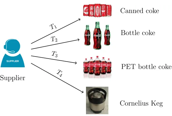
of JRP where products are ordered in large batches (e.g., coke), then packaged into various types of containers (e.g., canned coke, bottle coke, PET bottle coke, and Cornelius keg). An example is illustrated in Figure 1.1.3. The fixed cost involves a major setup cost for the order of the product (e.g., coke) and a minor setup cost for each of the items to be packaged (e.g., canned coke, bottle coke, PET bottle coke, and Cornelius keg).

(17)

Replenishment Cycle Time

Supplier

Canned coke

Bottle coke

PET bottle coke

Cornelius Keg

T1

T2

T₃ T₄

Figure 1.1.3: An example of joint replenishment

the total cost compared to EOQ models for a single item approach considering a set of twenty items.

Our research is motivated by the increase in operational complexity nowadays. The pervasiveness of JRP in actual practice, combined with its computational complexity, has long attracted researchers’ attention. Our goal is to help companies that are seeking to implement strategic inventory management and enhance their flexibility in a competitive environment for supply chain management.

1.2 Research Topics and Potential Contributions

(18)

Figure 1.1.4: Behavior of inventory in joint replenishment

cycle time to minimize the total costper unit time.

1.2.1 The Joint Replenishment Problem

The Joint Replenishment Problem (JRP) is concerned with the determination of lot sizes and schedule a group of items in single-facility production/inventory systems over an infinite (and continuous) planning horizon. The objective of JRP is to minimize the total costs incurred per unit time. The costs include setup costs and inventory holding costs. Two types of setup costs are considered in JRP:

1. A major setup cost is incurred whenever the production facility sets up to jointly replenish a subset of products.

(19)

and packaged).

It is noted that the major and minor setup costs are usually independent of the quantities of the items jointly replenished. When we solve the JRP, an intuitive move is to jointly replenish as many as items and share the major setup cost to minimize the average total cost.

The following assumptions are made in the JRP:

(i) The replenishment cycle time for each item equals to a integer multiple times the basic cycle time.

(ii) Demand rate is known and constant. (iii) Shortages are not allowed.

(iv) Replenishment can be done instantaneously.

(v) The planning horizon is infinite.

The parameters and decision variables are listed below: Parameters:

A0: major set up cost

ai: minor set up cost for itemi

di: demand rate for item i

hi: unit holding cost for itemi per unit time Decision Variables:

(20)

ki: multiplier of basic cycle time for itemi

The average total cost function AT Ci(ki, B) for itemi is characterized by

AT Ci(ki, B) =

ai

kiB

+ hidikiB

2 .

The mathematical model of JRP is

min ki,B

A0

B +

n X

i=1

AT Ci(ki, B) s.t. ki ∈N,∀i∈ {1,2,· · · , n}

B ∈_R, B >0,

which is a mixed integer nonlinear programming problem.

Motivated by incorporating relevant industrial concerns, our work will focus on JRP and its extensions including districting problem and cycle time constraints.

1.2.2 Joint Replenishment Problems under Cycle Time

Con-straints

Recently, there has been a shift in attention from the conventional JRP to the one under constraints (C-JRP) because even it is beneficial to exploit the economies of scale, companies still face some challenges when scheduling inventory planning. For example, the order quantity, delivery frequency, or storage capacity, are quite restrictive. As a result, the JRP would become more feasible and reasonable by taking account of these practical issues and limitations.

(21)

examples for the former ones include workforce capacity, storage space, the design of con-tainers and inventory investment. Examples for the later ones take account of machine capacities or raw material availability for the manufacture of product families. There are also some practical applications presented in the literature. [72] considered the C-JRP under some shipment policies in a food company in Thailand. The restrictions include not only the budget constraint and capacity constraint, but also the dependency of items and defective items in each shipment to maintain food quality and safety. On the other hand, concerning the lower bound constraints, [67] presented a case study in which a company that sells gift items in the Netherlands and Belgium managed their inventory system under the minimum order quantity (MOQ) constraints, e.g., M OQ = 10,000. Constrained joint replenishment and other types of inventory policies are tested in a simulation model with real data.

However, the problems and examples mentioned above are usually limited to certain types of constraints considering either upper bounds or lower bounds. In our study, we considered the JRP allowing for both upper bounds and lower bounds on the cycle time for each product, so our model is quite general and can be extended to C-JRP under various constraints.

The mathematical model for the C-JRP is modeled as follows:

min ki,B

A0

B +

n X

i=1

AT Ci(ki, B)

s.t. kiB ∈[Li, Ui],∀i∈ {1,2,· · · , n}

ki ∈N,∀i∈ {1,2,· · · , n}

B ∈_R, B >0,

(22)

respec-tively. Under the assumption that the demand rates for all items are constant, we can transform other types of resource constraints into cycle time constraints.

Since the solution approaches used to solve the conventional JRP is not applicable, we design a new search algorithm to solve the C-JRP. Based on the optimality solution structures, we categorize the items into four types and develop several theorems as the foundations of our search algorithm. The numerical experiments show that our proposed algorithm is effective by comparing the existing approaches in the literature.

This study contributes to the existing research in the following aspects:

(i) We formulate a mathematical model for the JRP under the cycle time constraints for each item.

(ii) Based on the junction-point analysis, we categorize the items into four types and prove some essential properties of the specific optimality structure.

(iii) While most of the research focused on how to design a heuristic algorithm to find a near-optimal solution, we develop an efficient algorithm to obtain a global optimal solution.

(iv) Numerical experiments are demonstrated to verify our proposed algorithm and support the theoretical findings and managerial insights.

1.2.3 Multi-Customer Joint Replenishment Problem with

Dis-tricting Consideration

(23)

extended version of JRP is called amulti-customer joint replenishment problem (MJRP), which aims to determine the lot-size and the replenishment schedule of multiple items of goods for multiple customers such that the average total cost is minimized over an infinite planning horizon.

Furthermore, when many customers scattered in a wide area, some practical consid-erations, such as geography, transportation or fleet size, may require us to divide them into some mutually exclusive zones in the planning region. Then, MJRP is employed to coordinate the replenishment for customers in the same zone. In general, customers in the planning region may be partitioned using zip codes or an official definition of dis-tricts. However, we would further consider the districting problem rather than using the given partitions. We call the integrated problem a multi-customer JRP with districting consideration (MJRPDC), which determines an optimal districting setting such that the average total cost of MJRP of all zones is minimized.

MJRPDC is of particular importance to a company that outsources the transportation and delivery operations to a third-party logistics (3PL) service provider. [70] indicated that by contracting-out to a 3PL provider with the right capabilities and resources, companies could focus on their core competency and leverage logistics to improve the service level. As of 2014, eighty percents of Fortune 500 companies and ninety-six of the Fortune 100 companies used some forms of 3PL services; see [63].

(24)

deci-sion which usually belongs to a tactical level decideci-sion rather than a strategic one; see, [90] and [46]. Strategic districting decisions that share some similarity with strategic location decisions, have a significant impact on the logistics operations and the relevant costs, e.g., routing and shipments costs. However, tactical inventory replenishment decisions should be taken into accounts in the strategic planning phase to avoid leading districting decisions to the sub-optimality since their related costs like setup and inventory holding costs could play important roles.

Before signing an outsourcing contract with the 3PL service provider, a company needs to provide a zoning plan and a replenishment schedule to cover all customers in order to negotiate a freight rate in the contract. To come up with a zoning plan, we may consider a districting problem that divides individual units into clusters, (called districts) according to some relevant planning criteria [48]. [82] provided some commonly used principles:

(i) Contiguity: A zone is said to be contiguous if it is possible to travel between any two territorial units without leaving the zone.

(ii) Population equity: A partition is said to be in population equity, if the number of desired units such as eligible voters and sales potential in each zone is about the same.

(iii) Compactness: A zone is said to be compact if it is geographically round-shaped.

In our study of MJRPDC, the population equity and compactness criteria are explicitly considered in the constraints.

(25)

MJRP under the general-integer (GI) policy. Then we design a GA-based framework to solve the districting problem using the proposed search algorithm to evaluate the performance of each districting setting. A numerical example of MJRPDC for a bank company is employed to demonstrate the proposed solution method. We also conduct some sensitivity analysis of the parameters corresponding to the demand equity and compactness criteria.

This study has at least three contributions:

(i) An efficient search algorithm for solving MJRP under the GI policy is proposed.

(ii) By incorporating the search algorithm for MJRP, we propose a GA-based solution method for solving the MJRPDC.

(iii) We use a bank company example to show some managerial insights and strategic implications that can be a guideline for a decision maker when signing a contract with 3PL service providers.

1.3 Outline of the Dissertation

(26)

(27)

Chapter 2 Literature Review

The lot-sizing problem has received wide attention both in academic literature and in practice because the inventory levels and structures may directly influence item avail-ability and core competence in terms of customer service. In this dissertation, we focused on the joint replenishment problem and its extensions with deterministic demand char-acteristic.

2.1 Lot-Sizing Problem

(28)

T CEOQ(Q) =

SD

Q +

Q

2h.

It is obvious that the T C(Q) is convex with respect to Q, so we can derive a global minimum

Q∗_EOQ = r

2SD

h ,

and obtain the minimized objective value, T CEOQ(Q∗) =

√

2SDh.

The economic itemion quantity (EPQ) model developed by [97] is similar to the EOQ model. The difference is that the EPQ further assumes that orders do not arrive all at once but receive incrementally at the itemion rate, P units per unit time (P > D). The total average cost T C is:

T CEP Q(Q) =

SD

Q +

Q

2h

1−D P

,

and the optimal order quantity

Q∗_{EP Q}= s

2SD h 1− D

P .

(29)

machine, one must decide: what to produce, what is lot size for each item and when should each lot be produced. Detailed reviews of the above models can be found in [24]. Another research stream is the extensions on the setup costs in the EOQ model. The

joint replenishment problem (JRP) is considered when there are not only setup costs for individual items but also a major setup for any lot is ordered. The JRP has been proven as an NP-hard problem and deserved further investigations due to the industrial prevalence. In this dissertation, we focused on the optimality structures of the JRP and its extension problems. In Section 2.2, we reviewed the JRP research and the methodologies have been done so far. Followed by Section 2.3, the literature about the JRP extensions is studied. Lastly, In Section 2.4, we examined the literature discussed the zone design and districting problems.

2.2 The Joint Replenishment Problem

The JRP has been heavily investigated since the early work of Shu[91], Goyal[32], and Silver[93]. The problem was proved to be NP-hard by Arkin et al.[3] and [17]. Due to its combinatorial nature, many different solution approaches have been proposed to solve the JRP faster and efficiently.

In the past studies, two main streams of strategies for the JRP are [52]: (i) Direct Grouping Strategy (DGS)

(ii) Indirect Grouping Strategy (IGS)

(30)

setup cost is high, the IGS is more efficient than the DGS; on the other hand, when the ratio is lower, the performance of DGS is better ([103][52]). To address the effect of the joint replenishment, in this study, we focused on the IGS.

Under the IGS the cycle time for item i is required to be:

Ti =kiB,

where ki ∈ N,∀i and B ∈ R. The policy defined by the basic cycle time and a set of multipliers is also known ascyclic policies. The order quantity for item iis

Qi =TiDi =kiBDi,

and the average total cost is

AT C(ki, B) =

A0

B +

n X

i=1

ai

kiB

+hidikiB 2

. (2.2.1)

The mathematical model for the JRP is formulated as follows:

min ki,B

AT C(ki, B)

s.t. ki ∈N,∀i∈ {1,2,· · · , n}

B ∈_R, B >0.

(31)

In the deterministic demand model, Goyal ([30] [32]) proposed an approach to enu-merate the combination of the basic replenishment cycle time B and the multiples of the basic cycle time of itemi,ki. The idea is that for a given set ofK = (k1, k2,· · · , kn)∈Nn, the optimal solution to

min

B>0AT C(K, B)

is given by

B(K) = v u u t

2A0+

Pn i=1 ai ki Pn

i=1kiDihi

.

It is obvious that when K = (k1, k2,· · · , kn)∈Nn increases, B(K) decreases. Therefore, [32] showed that for every K = (k1, k2,· · · , kn)∈Nn,

B(K)≤

v u u t

2A0 +

Pn i=1 ai ki Pn

i=1kiDihi

. (2.2.2)

The inequalities (2.2.2) also point out the upper bound of B. Also, for the strict cyclic policies, [32] proposed a lower bound ofB:

Bopt ≥ min

1≤i≤n r

ai

hiDi

. (2.2.3)

Using the upper bound and lower bound, Goyal developed an enumerative algorithm to identify all the local minimums. The objective is to reduce the number of combinations and obtain a global optimal solution. [103] derived another algorithm and showed that the method in [32] did not always lead to the optimal solutions and may be computationally difficult when the problem size is large. A new lower bound suggested by [105] is

Bv_min = 2A0

(32)

where T CU _{is a total cost upper bound which may update in the computation process.} [27] tried to enhance the efficiency of [32] enumeration algorithms with tighter bounds on the optimal values ofB. [106] later suggested a modification to ensure that [27]’s method can always guarantee the optimal solutions.

To increase the efficiency of enumerative algorithms, researchers also designed several heuristic algorithms. Silver [93] developed a non-iterative procedure. Kaspi and Rosen-blatt [51] later modified the heuristic algorithm. They proposed an algorithm called RAND which compared possible values between the minimum and maximum cycle times and then applying Silver’s improved algorithm at each cycle time. The RAND procedure is presented below:

The RAND algorithm

Step 1: Compute the upper bound Bmax and lower bound Bmin using (2.2.2) and (2.2.3).

Step 2: Divide the range (Bmin, Bmax) into m different, equally spaced, values ofB. (The value ofm is determined by the decision-maker)

Set j = 0.

Step 3: Set j =j+ 1. Set r = 0.

Step 4: Set r =r+ 1.

ForBj, and each item i, compute

k_i,r2 = 2aiB

2

j

Dihi

(33)

Step 5: Find k∗_i,r for each i, where

k_i,r∗ =L, if L(L−1)< k_i,r2 ≤L(L+ 1) (2.2.6)

Step 6: Compute a new cycle time Bj according to

Bj = v u u t

2A0+Pn_i₌₁ _ka∗i i,r

Pn

i=1Dihik

∗

i,r

. (2.2.7)

Step 7: If r = 1 or k∗_i,r6=k_i,r∗ ₋₁ for any i, then go to Step 4. Compute TC for this (Bj, k∗1,r,· · · , k

∗

n,r). If j = m, output the minimum value of

T C; otherwise, go to Step 3.

The RAND Algorithm was considered the best algorithm in terms of the solution quality and computation efficiency at the time. Therefore, it is usually viewed as a benchmark to verify a new algorithm.

(34)

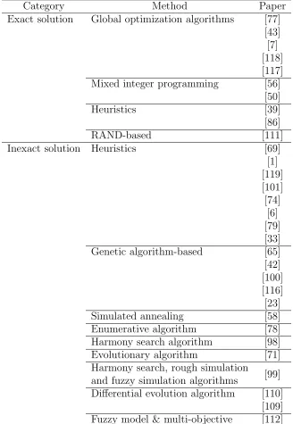
Table 2.1: Solution approaches for deterministic demand models

Category Method Paper

Exact solution Global optimization algorithms [77] [43] [7] [118] [117] Mixed integer programming [56]

[50]

Heuristics [39]

[86]

RAND-based [111]

Inexact solution Heuristics [69]

[1] [119] [101] [74]

[6] [79] [33] Genetic algorithm-based [65] [42] [100] [116] [23]

Simulated annealing [58]

Enumerative algorithm [78] Harmony search algorithm [98] Evolutionary algorithm [71] Harmony search, rough simulation

and fuzzy simulation algorithms [99] Differential evolution algorithm [110]

(35)

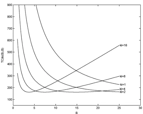
Figure 2.2.1: TheAT CP oT(ki(B), B) cost function

Also, it is a trend to adopt hybrid algorithms due to the potential complementary different methods can achieve better quality solutions. Here we list some exact and inexact solution approaches proposed in deterministic demand models in Table 2.1.

Most of studies discussed the JRP undergeneral integer (GI) policy. i.e., the multiples of basic cycle time for each item, ki, are positive integers, for all item i. [45] introduced a power-of-two (PoT) policy to the JRP where the multipliers, ki, are restricted to be

ki = 2p, p= 0,1,2,· · ·. One may formulate the mathematical model for the JRP under PoT policy as follows:

min ki,B

AT CP oT(ki, B) =

A0

B +

n X

i=1

ai

kiB

+ hidikiB 2

s.t. ki = 2p, p∈Z+,∀i

B ∈_R, B >0.

The plot of the objective function AT CP oT(ki(B), B) is shown in Figure 2.2.1.

(36)

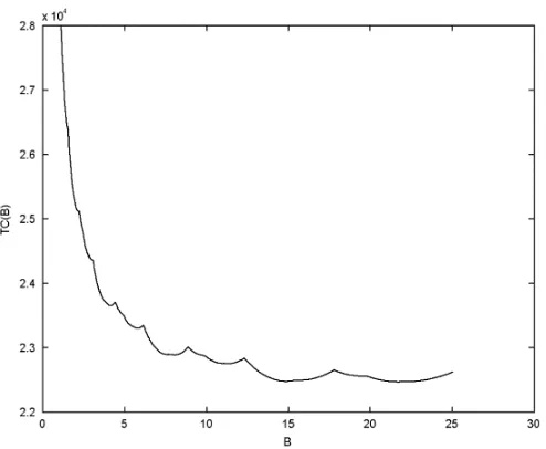
Figure 2.2.2: TheAT CP oT(B) cost function

policies. [85] further improved the difference to less than 2%. Lee and Yao [55] proposed a global optimum search algorithm for the JRP under PoT policy and guaranteed the global optimal solution.

Define

AT CP oT(ki, B) =

ai

kiB

+hidikiB

2 ,

and

AT C_{P oT,i}(B) = min ki

AT CP oT(ki, B),

AT CP oT(B) can be expressed as follows:

AT CP oT(B) =

A0

B +

n X

i=1

AT C_{P oT,i}(B).

(37)

B. Figure 2.2.2 is an example of AT CP oT(B) cost function. Next, they introduced the “junction points” which assists us to locate the optimal set of k0_is when searching along

B. The junction point of item i whenki = 2j, j ∈Z+ is presented as:

δi(2j) = 1 2j

r

ai

hidi

.

An efficient search algorithm based on the junction point structure is proposed to find a global optimal solution for the JRP under PoT policy.

Algorithm 1 The K-PoT Search Procedure:

for i= 1,· · · , n do

Set found=0 andj = 0

if B >q ai

hidi then

found ←0.

end if

while found=0 do

j =j+ 1.

if B > ₂1j

q ai

hidi then

found ←1.

end if end while

Set k_i∗(B) = 2j_.

end for

1. Initialize the search by:

(a) Locate T_cc∗ by the common cycle approach formula in Eq. (2.2.8).

T_cc∗ = s

2 (A0 +

Pn i=1ai) Pn

i=1hidi

(38)

Set l= 0 and

w0 = min{δi(ki) :δi(ki)> Tcc∗}.

If there exists no such w0, we set l = 1, w0 = Tcc∗, ˘K1 = {1,· · · ,1}, and

compute AT CP oT

˘

K1, Tcc∗

.

(b) Secure KP oT(Tcc∗)≡ KP oT(w0) by the K-PoT search procedure in Alg. 1, and

obtain

π = arg max

i {δi(ki)< w0}. Letw1 =δπ(kπ), and j = 1.

Check: If ˘B(KP oT(Tcc∗)) ∈ [w1, w0], set l = 1, ˘K1 = KP oT(Tcc∗), ˘Bl = ˘B( ˘Kl), and compute AT CP oT

˘

Kl,B˘l

.

2. Proceed to the next junction point wj and do the followings:

(a) Compute KP oT(wj) by KP oT(wj)≡KP oT(wj−1)\ {kπ} ∪ {2kπ}. (b) Obtain π = arg maxi{δi(ki)< wj}, and let wj+1 =δπ(kπ).

(c) Check: If ˘B(KP oT(wj))∈[wj+1, wj), setl=l+1, ˘Kl =KP oT(wj), ˘Bl = ˘B( ˘Kl), and compute AT CP oT

˘

Kl,B˘l

.

3. Let j =j + 1. Ifwj <

˘

B1

2 , then go to step 4; otherwise, go to step 2.

4. Secure the global optimal solution by (K_{P oT}∗ , B_{P oT}∗ ) = arg mini n

AT CP oT

˘

Kl,B˘l o

(39)

2.3 The Extensions of the JRP

It is observed that there has been a general trend of the JRP extensions. For example, the JRP has been applied in the supply chain management problems such as freight con-solidation, full truck-loads ,and joint delivery orders. ([31] [54] [11] [66]). In this section, we studied the literature of four topics: (1) the constrained JRP, (2) multi-customer JRP, (3) integrated JRP and (4) districting problem.

2.3.1 Constrained Joint Replenishment Problem

Unlike a conventional JRP, a constrained JRP (C-JRP) further takes some constraints into account. [31] first introduced the JRP with budget constraints and solved by a heuris-tic approach based on the Lagrangian multipliers method. [53] compared the performance of the genetic algorithm (GA) and RAND for solving the C-JRP. They indicated that the GA could handle C-JRP by introducing the penalty technique. Later, [65] also studied a JRP with a budget constraint. [115] dealt with the JRP under the warehouse-space restrictions in a distribution center. [1] worked on the JRP under budget limitations and proposed a heuristic framework based on linear programming. [72] considered the JRP with defective items and several restrictions such as shipment, budget, and transporta-tion capacity constraints. They compared the GA and the differential evolutransporta-tion (DE) algorithm to determine the reordering policy.

For the study that considers the upper bound constraints, [43] included the issues of storage capacity, transport capacities, and budget limitation in the conventional JRP.

mi: number of full truck load for an item i in an order

(40)

gi: maximum storage capacity of item i

ci: investment per unit of item i

Ci: the highest amount invested for item i

(PH) min

ki,B

AT C(ki, B) = A_B0 +Pni=1

ai+mit

kiB +

hidikiB

2

s.t. kiBdi ≤gi,∀i∈ {1,2,· · · , n}

kiBci ≤Ci,∀i∈ {1,2,· · · , n}

ki ∈N,∀i∈ {1,2,· · · , n}

B ∈_R, B >0.

(2.3.1)

On the other hand, [77] considered the JRP with minimum order quantities (MOQ), and adapted [113]’s formulation to solve it. The problem is formulated as follows:

(PP D) min

ki,B

AT C(ki, B) = A_B0 +Pn_i₌₁ hidi₂kiB

s.t. kidiB ≥M OQi,∀i∈ {1,2,· · ·, n}

ki ∈N,∀i∈ {1,2,· · · , n}

B ∈_R, B >0.

(2.3.2)

They derived proper lower and upper bounds for the basic cycle time with a correc-tion factor and showed that the algorithm can always obtain a global optimal solucorrec-tion. However, considering the complexity of C-JRP, most researchers attempted to develop heuristic algorithms to obtain an approximated solution rather an optimal one.

In this study, we would like to include the cycle time constraints,

kiB ∈[Li, Ui],

(41)

quantities considered in [77]. Since the demand rate for each item is constant, we can transform the M OQinto Li by

Li =

M OQ di

,∀i.

Refer to [43], the upper bound constraint may result from the storage capacity or budget limitation. The cycle time upper bound with respect to the maximum storage capacity is

U_ig = gi

di

,∀i,

where gi is the maximum storage capacity of item i. On the other hand, the cycle time upper bound related to the budget limitation is

U_ic= Ci

cidi

,∀i,

where Ci is the highest amount invested for item, and ci is the investment per unit of item i. We then set

Ui = min{Uig, U c i},∀i.

(42)

2.3.2 Multi-Customer Joint Replenishment Problem

The replenishment of multi-customers is a common context within the operation envi-ronment, so companies are seeking models to make decisions on inventory management that result in efficient MJRP solutions ([86] [107] [13] [87]). However, it is an area that has received little attention in the literature.

[57] solved the MJRP with the RAND method. [12] considered an application of the multi-customer JRP in which a leading bank in Hong Kong replenished forms for the branches (treating them as “customers”). The bank divided all branches into eight groups (corresponding to eight predetermined routes), and practiced joint replenishment of items (i.e., the forms for their daily operations) among the branches in the same route (as depicted in Figure 2.3.1). The authors solved the multi-customer JRP by a modified GA given the eight groups of branches. However, they ignored the districting problem, namely, how to come up with the eight delivery zones, but only attempted to minimize the average total cost of the multi-customer JRP in each zone. Different from their study, we would further consider how to partition customers into a fixed number of groups instead of given the partitions.

2.3.3 Integrated Joint Replenishment Problem

(43)

Figure 2.3.1: The scenario in [12] with predetermined routes

this problem. [89] investigated the same problem and reformulated the problem as a linear integer set-covering problem. [90] further extended to the case taking into account the routing decisions.

Different from the studies mentioned above, Silva and Gao [92] focused on the joint replenishment inventory-location problem, and formulated it as a fixed charge location problem (FCLP) with its objective function including location-specific costs and replen-ishment costs. However, in our study, since we do not set up any facility, so there is no fixed cost to open a facility. The centroid of each zone is only a virtual location rather than a physical one.

Some studies integrated the JRP with delivery decisions in the literature, e.g., [11] [16], [80], [14]. However, since the firm outsources the delivery operations to a 3PL service provider in our study, we do not include transportation costs in the objective function of the proposed model.

(44)

al.[12], but the decision-making scenario is significantly different from other location and inventory problems or JRP considering delivery. Therefore, we are motivated to formulate a mathematical model and propose an effective solution approach based on GA for solving the MJRPDC in this study.

2.4 Districting Problem

When many customers scattered in a wide area, it may be necessary to divide them into different (and mutually exclusive) zones in the planning region due to some practical issues, such as geography, transportation or fleet size concerns. Districting problem aims is to determine which customers should order together according to relevant planning criteria. In this section, we reviewed some important districting criteria, applications, and solution approaches.

2.4.1 Districting Criteria

According to [82], the decision-makers usually consider the following issues when solving the districting problem.

(i) Contiguity: A zone is calledcontiguous if it is possible to travel between the terri-torial units without ever leaving the zone.

(ii) Population equity: The decision-makers desire population equity concerning differ-ent performance measure, e.g., eligible voters, sales potdiffer-ential, and any combinations of them.

(45)

(iv) Integrity: Each customer is assigned to exactly one district.

Here are some examples of integrity: The complete and exclusive assignment in po-litical districting and school districting are apparent. In sales territory design, a unique allocation results in clear responsibilities for the sales force avoiding contentions and allowing the establishment of long-term customer relations. Next, we will explain the applications of the districting problem and how the criteria are considered.

2.4.2 Applications

The districting problems have been widely applied in different areas such as electoral dis-tricting ([44][40][82]), school disdis-tricting ([25][88]), and sales territories ([26][121]. Depend-ing on the practical context, districtDepend-ing is also called territory design, territory alignment, zone design, or sector design [48]. In each context, districting serves a different purpose and could significantly impact the performance of the operations.

For example, inelectoral districting problem, it is essential for the designer to maintain districts neutral and avoid gerrymandering. No political party should be able to take advantage of the electing subdivision in order to gain more citizens’ votes. For political districting, the integrity criteria are obvious. The population equity criterion is employed to ensure the “one-person-one-vote” principle [48]. The sum of the populations in any district should lie within a predetermined range such that the population units in the district are not far from each other. To satisfy the compactness requirement, [62] assigned the pairwise sum of the Euclidean distance between population units in a district as the penalty cost for the district.

(46)

not violate the individual school capacities and racial balance limitations. According to [88], the problem can be stated as follows: “Minimize the total weighted distance traveled in the school system subject to the constraints that: all students are assigned to schools, assignments do not violate the individual school capacities to accommodate students, and that a balance between minority and majority students assignments at each school be maintained within some pre-specified allowable range.” Therefore, the capacity of schools and the balancing of minority and majority are various considerations of “equity” principle. In order to create compact districts, no student should travel more than a specified maximum distance. Following this constraint, the resulting patterns will be consolidated rather than spread out. Furthermore, school sectors should be contiguous to allow students from the same neighborhood to be assigned to the same school. The contiguity of the sectors also facilitates school bus routing schedule.

In marketing applications, the sales territories problem ([26], [121]) indicates that each salesperson has a particular sales territory, and the territories may not overlap. To design compact sales territories, they minimize the weighted distance between the areas and the territorial centers. This aim can also implicitly lower the driving cost of visiting customers. To design balanced sales territories, the sales potential and the anticipated workload should be as uniform as possible, e.g., in a specific range which is the mean size plus or minus a tolerance. Therefore, the districting of sales territories take into account not only the “compactness” but also the “equity” principles.

2.4.3 Solution Approaches

(47)

([38][26][29][59]), or set partitioning ([28][62]), and others utilized computational geome-try methods ([120][49][83]) or construction methods ([104][8]). One may refer to [48] for a comprehensive survey of the solution approaches for the districting problems. Among all these approaches, we observe that it is usually difficult to embed the contiguity and compactness properties into a rigid and concise mathematical model.

The concept of “zone centroid” for clustering was introduced to solve the districting problems in the literature. According to [4], two approaches are popular in determining the candidate centroids: either restricts each zone center to be one of the customer’s loca-tion or not. We reviewed two common approaches: localoca-tion-allocaloca-tion method and genetic algorithm where the former one restricts each zone center to be one of the customer’s location, but the latter one does not.

Location-allocation method

[38] proposed the first mathematical programming approach and applied to the political districting problem. It aims to partition all basic unitsJ into a number ofpdistricts and locate a center within each district such that the partition satisfies the planning criteria of balance and compactness. To achieve the demand equity, researchers suggested an allowance relative deviationα >0 of the demand amount from the mean district amount

µ. [38] modeled the problem as a capacitated p-median facility location problem. Let J

be the set of all customers, and,

dj: demand rate for item j

(48)

min X i,j∈J

djwij2xij (2.4.1)

s.t.X

i∈J

xij = 1, ∀j ∈J; (2.4.2)

X j∈J

djxij ≥(1−α)µyi, ∀i∈J; (2.4.3)

X j∈J

djxij ≤(1 +α)µyi, ∀i∈J; (2.4.4)

X i∈J

yi =p, (2.4.5)

yi, xij ∈ {0,1}, ∀i, j ∈J, (2.4.6)

where xij = 1 if customer j is assigned to center i, 0 otherwise, and yi = 1 if customer

i’s location is selected as district center, 0 otherwise. The objective function (2.4.1) min-imize the distance from each customer location to its zone center which also implies to maximize the compactness. Constraints (2.4.2), together with xij ∈ {0,1} model the unique and exclusive assignment criterion. Constraints (2.4.3) and (2.4.4) mandate the demand equity principle by assuring that the total demand of all the customers in each zone cannot exceed an allowance relative deviationα >0 of the demand amount from the mean district amountµ. Constraints (2.4.5) ensure that exactlypcustomer locations are selected as district centers. Finally, constraints (2.4.6) define the domain of the decision variables. Note that the centers are just required to evaluate district compactness instead of setting up real facilities.

(49)

zone centers, and (2) anallocation phase to allocate demand to the zone centers. We first determine the initial locations of the zone centers. Once the centers have been fixed, the allocation phase determines a balanced assignment, then based on the group of customers in each zone, we relocate the zone center in the location phase such that the compactness is maximized. The two phases are alternately performed until a satisfactory result is obtained.

Genetic algorithm

To deal with the increase in flexibility and complexity, many researchers adopt heuristic or meta-heuristic approaches for solving the districting problems. For example, simulated annealing ([60][73][21]), tabu search ([73][81][8]), and genetic algorithm (GA) ([19],[61]). [114] presented a thorough survey in this line of study.

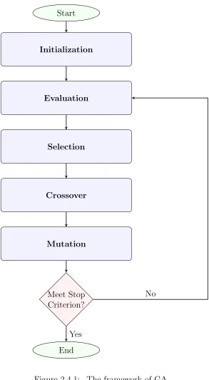
GA introduced by [41] is a meta-heuristic method inspired by the process of natu-ral selection. It reflects the process of natunatu-ral selection where the fittest individuals are selected to produce offspring of the next generation. An individual is characterized by a set of parameters (variables) known as genes. Genes are joined into a string to form a chromosome (solution). The set of all chromosomes is known as the population. Chro-mosomes in a population are evaluated based on their fitness value in order to evolve a new population ,and this process or iteration is called ageneration. The operators in GA include evaluation, selection, crossover, and mutation. Over successive generations, the population “evolves” toward an optimal solution. The framework of GA is depicted in Figure (2.4.1).

(50)

the sum of a set of calculated parameters related to the problem domain can be used as the fitness function. As part of the evaluation process, the elite chromosome of the generation is determined.

• Selection: Selection in GA determines the chromosomes being chosen from a pop-ulation in the last generation to undergo genetic operators before forming the popu-lation in the next generation. Theroulette wheel method is one of the most popular ways in which proportions of the wheel depending on the fitness values of chromo-somes, so chromosomes with better fitness values would have greater opportunities of survival than the weaker ones.

• Crossover: The crossover operator combines the features of the two given solution strings to form new solution offspring. The crossover rate is specified by the users.

Two-point crossover is adopted in our study where two crossover points are picked randomly from the parent chromosomes. The bits in between the two points are swapped between the parent organisms.

• Mutation: Mutation is usually viewed as a way of small random deviation and diversity in the evolutionary process because it alters one or more gene values randomly in a chromosome before being sent to the next generation. It helps to raise the diversity and exploit the solutions in its neighborhood when chromosomes may become similar to each other close to the end of the search.

The GA terminates when no improvement shows in the evolutionary process. For example, our GA procedure terminates when the best-on-hand solution was not updated over a certain number of generations.

(51)

Start

Initialization

Evaluation

Selection

Crossover

Mutation

Meet Stop Criterion?

End

No

Yes

(52)

Binary encoding is the most common method mainly because it is first introduced and it is relatively simple. [75] used the GA to find a near-optimal partitioning of the given data and set it as an initial seed value in theK-mean algorithm which is used to optimize total within-group sum of squared error. By relaxing the restriction that each zone center has to be one of the customer’s location, it is more flexible to meet the compactness criterion when solving the districting problem.

Furthermore, they assumed that the efforts or costs of transportation within a maxi-mum allowed unit distance, uare negligible. As a result, the search space can be signifi-cantly reduced from a continuous space into a reasonable number of discrete grid points

with a unit of grid width/length being no more than u km. We denote the minimum number of grids needed to represent the coordinates of the service region in l−axis as

GPl as Eq. (2.4.7), l∈ {x, y}.

GPl=

lmax−lmin

u

, (2.4.7)

where lmin and lmax are the largest and smallest coordinate values, respectively, of the locations of the customers in the l−axis, l ∈ {x, y}.

Let Bl be the number of bits required for the representation in thel−axis:

Bl =dlog2(GPl+ 1)e, (2.4.8)

where l∈ {x, y}. Following Eq. (2.4.7) and (2.4.8), we are able to guarantee thatul, the grid width/length in the l−axis, is no larger than u as

ul =

lmax−lmin

(53)

where l ∈ {x, y}. Now, we have an encoding mechanism to convert the coordinate value in the l−axis of a centroid into binary strings (bBlbBl−1· · ·b1b0) for the chromosome

representation in our GA. Its decoded coordinate value in the l−axis of a centroid, denoted as ˜l, can be obtained by

˜

l =lmin+ Bl

X i=0

bi·2i !

·ul (2.4.10)

∀l ∈ {x, y}. In this study, we would follow the encoding mechanism in [75].

(54)

Chapter 3 The Joint Replenishment Problems

under Cycle Time Constraints

3.1 Introduction

(55)

limitations.

The JRP is a classic problem in inventory management. The objective is to determine the optimal replenishment cycle time for each item such that the average total cost is minimized. The average total cost is composed of two parts: the setup (or ordering) cost and the inventory holding cost. The setup cost includes (i) a major setup cost, A0, for

collectively processing a subset of items; (ii) a minor setup costai for handling each item

i. Generally, these costs are regardless of the quantity replenished. On the other hand, the inventory holding cost is described as a percentage of the inventory value. It includes storage costs, related investment, taxes, and insurance.

Typically, the JRP assumes that the demand rate of each item di is known and constant, and each item i is replenished after a fixed cycle, denoted by Ti. Most studies suggest thatTiequals to a positive integer (ki) times a basic cycle time (B >0). Besides, it is assumed that the warehouse of the production/inventory system has infinite capacity, and the replenishment of each item is instantaneous. No shortage or back-order are allowed.

(56)

optimization and derived a tighter upper and lower bounds. [52] and [5] provided an overall review of the models, findings, and algorithms related to the JRP.

Some researchers investigated different order policies in the JRP. [55] considered the JRP under the power-of-two (PoT) policy where all the multipliers, ki, are restricted to be PoT integers, e.g.,ki = 2p, for somep= 0,1,2,· · ·. They proposed an effective search algorithm finding the global optimal solutions based on their “junction point” analysis on the optimality structure. In this study, we will conduct theoretical analysis based on junction point similar to [55] and propose a search algorithm to solve the C-JRP under

general integer (GI) policy where all the multipliers,ki, are restricted to be some positive (but, not necessary PoT) integers.

Most of the studies on JRP assumed that there are no limitations on the replenish-ment of all items. However, in practice, many constraints like transportation, budget and physical space usually impact significantly on inventory planning. According to [9], there are two types of resource constraints in production and inventory management: those over all items, and those over disjoint subsets of the items. Some examples for the former ones include workforce capacity, storage space, the design of containers and inventory in-vestment. Examples for the later ones take account of machine capacities or raw material availability for the manufacture of product families.

(57)

based on linear programming. [72] considered the JRP with defective items and sev-eral restrictions such as shipment, budget, and transportation capacity constraints. They compared the GA and the differential evolution (DE) algorithm to determine the reorder-ing policy. Different from the literature mentioned above, [77] considered the C-JRP with lower-bound restrictions on the replenishment lot. They adapted the formulations from [113] and applied to the problem of JRP with minimum order quantities (MOQ). They also derived proper lower and upper bounds for the basic cycle time with a correction factor and showed that the algorithm is able to obtain a global optimal solution.

There are also some practical applications presented in the literature. [72] considered the C-JRP under some shipment policies in a food company in Thailand. The restrictions include not only the budget and capacity constraint, but also the dependency of items and defective items in each shipment to maintain food quality and safety. Besides, [67] presented a case study in which a company that sells gift items in the Netherlands and Belgium managed their inventory system under the MOQ constraints, e.g., M OQ = 10,000. Constrained joint replenishment and other types of inventory policies are tested in a simulation model with real data.

However, the problems and examples mentioned above are usually limited to certain types of constraints considering either upper bounds or lower bounds. In our study, we considered the JRP allowing for both upper bounds and lower bounds on the cycle time for each item, so our model is quite general and can be extended to various constraints because the demand rates for all items are assumed constant. We will demonstrate the transformations of two numerical examples in literature in Section 3.2.2.

(58)

and proved some essential properties of the specific optimality structures. Furthermore, while most of the research focused on how to design a heuristic algorithm to find a near-optimal solution, we developed an efficient algorithm to obtain a global near-optimal solution. Lastly, numerical experiments and sensitivity analysis are demonstrated to verify our proposed algorithm and support the theoretical findings and managerial insights.

The rest of this paper is organized as follows. In Section 3.2, we introduced the decision-making scenario and formulated the C-JRP mathematical model. Section 3.3 derived some theoretical results based on the optimality structure and developed an efficient algorithm for solving this C-JRP. In Section 3.4, we compared our proposed algorithm with those in the literature. Also, some numerical experiments are conducted to verify the effectiveness of our proposed algorithm. In Section 3.5, we concluded the paper and discussed possible future research directions.

3.2 Mathematical Model

In this section, we first introduced the targeted problem, defined the notations and as-sumptions used throughout the paper, and then presented the mathematical model in Section 3.2.2.

3.2.1 Problem definition and notations

In this study, we investigated a constrained JRP where the replenishment cycle time (Ti = kiB) for each item i is restricted in the range of a lower bound and an upper bound, i.e., Li ≤ kiB ≤ Ui,∀i ∈ 1,2,· · · , n where n is the number of items, Li and

Ui represent the lower bound and upper bound of the replenishment cycle time of item

(59)

op-timal multipliers of all items (k₁∗, k₂∗,· · ·, k_n∗) such that the average total cost is minimized.

Notations

A0: major setup cost

• For every item i∈ {1,2,· · · , n}, we define the following notations:

di: demand rate

hi: inventory holding cost per item per unit of time

ai: minor setup cost

Li: lower bound of replenishment cycle time

Ui: upper bound of replenishment cycle time • The decision variables are listed as follows

B: basic cycle time

ki: multiplier of basic cycle time for item i

• For short notation, we define the optimal solutions by

B∗: optimal basic cycle time

k_i∗: optimal multiplier of basic cycle time for item i

Assumptions For each item i, we assume that (i) The replenishment cycle time is Ti =kiB. (ii) Demand rate is known and constant.

(60)

(iv) Replenishment can be done instantaneously.

(v) The planning horizon is infinite.

3.2.2 Model formulation

The unconstrained JRP (Pu_{) is formulated as follows:}

(Pu)

min

(k1,···,kn),B

AT Cu(ki, B) = A_B0 +Pni=1

ai

kiB +

hidikiB

2

s.t. ki ∈N,∀i∈ {1,2,· · · , n}

B ∈_R, B >0.

(3.2.1)

In this study, we would like to include constraints on the replenishment cycle time,

kiB ∈[Li, Ui],

for each item i.

The lower bound constraint,Li, is motivated by the minimum order quantities (MOQ) considered in [77]. Such a lower bound may also result from the design of containers used in the logistics operations of transportation or material handling. Since the demand rate for each item is constant, we can transform the M OQinto Li by

Li =

M OQ di

,∀i.

(61)

goods that could be flammable, radioactive, or explosive, etc. The upper bound on the replenishment cycle time with respect to the maximum storage limitation is

U_ig = gi

di

,∀i,

where gi is the maximum storage limit of item i. On the other hand, the upper bound on the replenishment cycle time related to the budget limitation is

U_ic= Ci

cidi

,∀i,

where Ci is the highest amount invested for item i, and ci is the investment per unit of item i. We set

Ui = min{Uig, U c i},∀i.

The JRP under cycle time constraints is formulated as a mixed-integer nonlinear programming problem:

(P)

min

(k1,···,kn),B

AT C(ki, B) = A_B0 +Pn_i₌₁

ai

kiB +

hidikiB

2

s.t. kiB ∈[Li, Ui],∀i∈ {1,2,· · · , n}

ki ∈N,∀i∈ {1,2,· · · , n}

B ∈_R, B >0.

(3.2.2)

For each item i, let AT C_i(B) be the average total cost taking the optimal and feasible value of multiplier ki atB, for all B >0.

AT C_i(B) = min ki∈Fi(B)

ai

kiB

+hidikiB 2

(62)

where

Fi(B) =      ki

Li ≤kiB ≤Ui

ki ∈N

     .

Then problem (P) is equivalent to:

min

B Φ(B) = A0

B + Pn

i=1AT Ci(B)

s.t. B ∈_R, B >0.

(3.2.4)

3.3 Theoretical Results and the Proposed Algorithm

3.3.1 Optimality structures for the unconstrained JRP

Before solving our problem (P), we first remove the cycle time constraints and investigate the structures of the optimal solutions of the unconstrained problem (Pu_{). Without} considering the major setup cost term in the objective function, the average total cost

AT C_iu(ki, B) for each item i can be expressed by

AT C_iu(ki, B) =

ai

kiB

+ hidikiB

2 ,∀i. (3.3.1)

For any given ki ∈ N, the function AT Ciu(ki, B) is strictly convex with respect to B, so we can secure a minimum objective value √2aihidi at B =

q ₂_a

i

hidik2i

. Therefore, the optimal solution of the function AT Cu

i (ki, B) can be defined as:

AT Cu_i(B)= inf∆ ki∈N

{AT C_iu(ki, B)|B >0}. (3.3.2)

(63)

con-secutive convex curves AT Cu

i (ki, B) and AT Ciu(2ki, B) concatenate on the curve of the

AT Cu_i(B) function. Similarly, under GI policy, a junction point is defined as a particular value of B where two consecutive convex curves AT Cu

i(ki, B) and AT Ciu(ki+ 1, B) con-catenate on the curve of theAT Cu_i(B) function. These junction points play an important role to determine at “what value ofB” one should change the value of ki in order to ob-tain the optimal value of the AT Cu_i(B) function. Using simple algebra, we could derive a closed form to locate the mth junction point,δi(m), for item i.

δi(m) = s

1

m(m+ 1) r

2ai

hidi

, m ∈_N. (3.3.3)

These junction points can be ordered decreasingly as δi(1) > δi(2) > · · · ,∀i. Given a value of B, we define ki(B) as the optimal multiplier that obtains AT Ciu(B). Suppose that ki(δ−) and ki(δ+) are the optimal multipliers of the left-side and right-side convex curves with regard to a junction point δ of the AT Cu_i(B), then ki(δ−) = ki(δ+) + 1. In other words, given any value ofB, the optimal multiplier ki(B) can be derived by

ki(B) =

−1

2+ 1 2

r

1 + 8ai

hidiB

, (3.3.4)

where dxe denotes the the ceiling function maps x to the least integer greater than or equal to x. (See also [113]).

3.3.2 Optimality structures for the constrained JRP

(64)

and the lower bound for each item. Givenki ∈N, one of the following inequalities would

stand. Case (1):

Li

ki+ 1

< Ui ki+ 1

≤ Li ki

< Ui ki

; (3.3.5)

or Case (2):

Li

ki+ 1

< Li ki

≤ Ui ki+ 1

< Ui ki

. (3.3.6)

In Case (1), the objective function AT C_i(B) is feasible only when B ∈_L_i m,

Ui

m

for some positive integermsuch that Li ≤mB≤Ui . Therefore, our search range of B is reduced to some intervals, e.g., [Li, Ui],

Li

2 ,

Ui

2

,· · ·. And, ki(B) is characterized as follows :

ki(B) =m, if B ∈ Li m, Ui m ; (3.3.7)

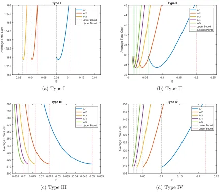
We call this kind of item Type I item. Figure 3.3.1(a) shows the feasible intervals of

AT Ci(ki, B) function for a Type I item. In Case (2): Li

ki+1 <

Li

ki ≤

Ui

ki+1 <

Ui

ki, the intervals

h Li

ki,

Ui

ki

i

and h Li

ki+1,

Ui

ki+1

i

are over-lapped given ki, so ki(B) is not easily obtained as in Case (1). Therefore, we further divided the Case (2) into three types: Type II, III, and IV. Before we investigate the characteristics of these three types, Lemma 3.1 describes some properties that would be saved for later.

Lemma 3.1. For each item i, if there exists m ∈ _N such that Li

m ≤δi(m) ≤ Ui

m+1, then

∀k ∈_N and k ≥m,

(1). Li

k ≤ q

1

k(k+1)

q

2ai

hidi

(2). q_k₍_k1₊₁₎q2ai

hidi ≤

Ui

(65)

0.02 0.04 0.06 0.08 0.1 0.12 0.14 B 182 182.5 183 183.5 184 184.5 185 185.5 186

Average Total Cost

Type I k=1 k=2 k=3 Lower Bound Upper Bound

(a) Type I

0 0.05 0.1 0.15 0.2 0.25

B 32 34 36 38 40 42 44 46

Average Total Cost

Type II k=1 k=2 k=3 k=4 k=5 Upper Bound Junction Points

(b) Type II

0.005 0.01 0.015 0.02 0.025 0.03 0.035 0.04 0.045 0.05 0.055 B 200 210 220 230 240 250 260 270 280 290 300

Average Total Cost

Type III k=1 k=2 k=3 k=4 k=5 Upper Bound

(c) Type III

0.05 0.1 0.15 0.2 0.25

B 105 110 115 120 125 130 135 140 145 150

Average Total Cost

Type IV k=1 k=2 k=3 k=4 k=5 Lower Bound Upper Bound

(d) Type IV

(66)

Proof.

(1). The lemma can be proved by mathematical induction. Let k =m+j. When j = 0, it works obviously. Assume, for j = n holds. q_m1₊_nq_m₊1_n₊₁q2ai

hidi ≥

Li

m+n is equivalent to

q

1

m+n+1

q

2ai

hidi ≥

Li

√

m+n, so q

1

m+n+1

q

1

m+n+2

q

2ai

hidi ≥

Li

√

m+n q

1

m+n+2 ≥

Li

m+n+1 which

implies j =n+ 1 holds.

(2). Let k=m+j. When j = 0, it works obviously. Assume, forj =n holds. r

1

m+n

r 1

m+n+ 1 r

2ai

hidi

≤ Ui

m+n+ 1

is equivalent to

r 1

m+n+ 1 r

2ai

hidi

≤ Ui

m+n+ 1

√

m+n,

so r

1

m+n+ 1 r

1

m+n+ 2 r

2ai

hidi

≤

r 1

m+n+ 2

Ui

m+n+ 1

√

m+n≤ Ui

m+n+ 2

which implies j =n+ 1 holds.

Now, we discussed the other three types, namely, Type II, III andIV, when Case (2) condition holds.

We denote an item as Type II when Li

m+1 <

Li

m ≤ Ui

m+1 <

Ui

m and q

1

m(m−1)

q

2ai

hidi ∈

Li

m−1,

Ui

m

hold for some positive integer m≥2. The interval of two consecutive junction points [δi(m), δi(m−1)] is within the interval of

Li

m, Ui

m

The Joint Replenishment Problem and Extensions.

ABSTRACT

DEDICATION

BIOGRAPHY

ACKNOWLEDGEMENTS

TABLE OF CONTENTS

LIST OF TABLES

LIST OF FIGURES

Chapter 1

Introduction

1.1

Motivation

1.2

Research Topics and Potential Contributions

1.2.1