Abstract
Sun, Xuejun
ULEDS-SVMs: Upper/Lower Limit and Error Data Supported Support Vector Machines
(Under the direction of Jon Doyle)
A Support Vector Machine, ULEDS-SVM, was developed for classification in data domains
which contain limits or errors.
Data with upper or lower limits are not the same as missing data. They may provide
con-straints at a certain level in data classification and modeling. Data with errors may be regarded
as the special co-existing case of an upper and a lower limit at the two boundaries of an
at-tribute. Data with such qualities widely exist, from scientific data measurements to databases
resulted from integration. Including these data in training rather than dropping them or
replac-ing them with some arbitrary value is desirable because they may provide useful constraints.
An enhanced 1R algorithm is described which may be able to handle a data domain that
contains limits and errors. However, the time complexity is
, where
is the number
of entities, the number of attributes, and
the number of elements in one attribute. This does
not allow good scalability.
Support Vector Machine (SVM) treatment of the data in such a domain is, however, very
an entity of data items is not trainable if the class, , and the normal of the separation plane,
, satisfy some conditions: an attribute exists such that ; ;
for an upper limit, lower limit and an error, respectively, where
and
are data at their centroid values, except for the th component which is located at
the upper and lower boundaries of an error, respectively. Untrainable data need to be dropped,
and trainable data need to be included in training.
By utilizing an intersection concept, which is the intersection of the separation plane and
the uncertain region of limit or error data, testing can be set to be correct if such an intersection
exists for limit or error data. Intersection conditions are determined by the existence of an
attribute, , for an entity such that
!
" for limits, or
" for
errors, where
$#
%
is the function of the separation plane, and
!
denotes the
upper (1) or lower (-1) limit at the th component. The prediction of class is meaningful for
those data without intersections.
An astronomical data set (CHDF-N) is integrated based on Chandra Deep Field (CDF)
and Hubble Deep Field (HDF) North observations. Some spectroscopic identifications are
available, but some are beyond the existing instrument limits. CHDF-N is used as a test bed for
the ULEDS-SVMs algorithms application implemented via Matlab. This classification may be
applicable to the study of the formation and evolution of galaxies in the deepest universe.
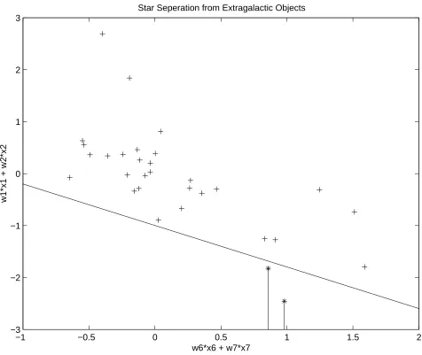
The separation of stars and extragalactic objects allows a 100% accuracy rate; however, the
separation would otherwise be ambiguous if the limit data in the extragalactic class were not
ac-curacy for the separation of galaxies and active galactic nuclei (AGNs). This rate is better than
the 72.4% accuracy rate attained using the conventional
plot separation method
commonly used in the astronomy community. The prediction rate increased from 49.6% using
ULEDS-SVMs: Upper/Lower Limit and
Error Data Supported Support Vector Machines
by
XUEJUN SUN
A thesis submitted to the Graduate Faculty of North Carolina State University
in partial fulfillment of the requirements for the Degree of
Master of Science
COMPUTER SCIENCE
Raleigh, North Carolina
2003
APPROVED BY
—————————————— ——————————————
——————————————
Biography
Name: Xuejun Sun
Education:
2002-2003 M.S., Computer Science, NC State University
2001-2002 Student for life long education program, Computer Science, NC State University
1984-1987 M.S., Physics, Graduate School, University of Science and Technology of China
1980-1984 B.S., Physics, Beijing Normal University
Research and visiting experiences:
1999-2001 Staff, Physics, University of Alabama in Huntsville
1998-1999 Visiting Scholar, Universities of Space Research Association/NASA Marshall Space
Flight Center
1997-1998 Visiting Scholar, Los Alamos National Lab
1996-1997 Staff, Beijing Astronomical Observatory, Chinese Acadamy of Sciences
1987-1996 Staff, Institute of High Energy Physics, Chinese Acadamy of Sciences
1994-1996 Visiting Scholar, Max-Plank-Institut f¨ur extraterrestresche Physik, Germany
ACKNOWLEDGEMENTS
The author is very grateful for the support and help of so many people during the time that he
conducted his research work and thesis preparation.
The author’s advisor, Dr. Jon Doyle, guided the Kernel Method direction for the author’s thesis.
His conversations were always inspirational and his encouragement accompanied the author’s
work throughout this research.
Dr. Shuangnan Zhang’s discussions with the author about the current status of major surveys in
astronomy helped the author to make the decision to choose Chandra and Hubble Deep Field as
the area for the Machine Learning application that uses the method developed in this research.
The confidence to work on this application was also encouraged by Dr. Dick Shaw.
The author’s interest in Machine Learning largely originated from communications with Dr.
Fenimore. His support and inspiration helped the author significantly, not only during the
author’s student life but beyond. Dr. Xiaohui Fan’s discussions with the author about the Slon
Digital Sky Survey strengthened the author’s ideas about the usefulness of a Machine Learning
method that features an upper limit and error handling capability.
Mr. Lloyd Williams and Ms. Mary K.S. Brown edited the author’s English. Mr. Brent Dennis
helped the author in LaTex.
The author’s wife, Toni, and daughter, Anna, encouraged the author throughout his graduate
study at North Carolina State University. Without their understanding and steadfast support he
Contents
List of Figures vi
List of Tables vii
1 Introduction 1
2 Enhanced 1R - A Simple Method to Treat Data with Limit and Error Attributes 6
2.1 1R Rule Extension . . . 8
2.2 Comments . . . 11
3 Mathematical Foundation for ULEDS-SVMs 13 3.1 Training . . . 13
3.2 Test . . . 20
3.3 Prediction . . . 21
4 Algorithms 25 4.1 Upper and Lower Limit Case . . . 26
4.1.1 Training . . . 26
4.1.2 Test . . . 29
4.1.3 Prediction . . . 30
4.2 Data With Error . . . 32
4.2.1 Training . . . 32
4.2.2 Testing . . . 34
4.2.3 Predicting . . . 34
4.3 ULEDS-SVMs . . . 35
5 Chandra and Hubble Deep Field North (CHDF-N) dataset 40 6 Classification via ULEDS-SVM on CHDF-N Dataset 46 6.1 Implementation of ULEDS-SVMs Incorporated with LSVM . . . 46
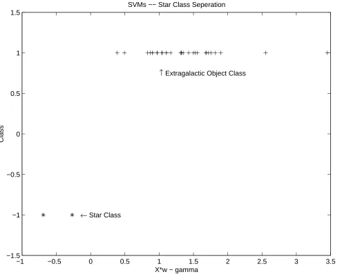
6.2 Classification of the Star Class . . . 47
6.3 Classification of Extragalactic Objects . . . 49
7 Discussion and Conclusion 59
7.1 Discussion . . . 59
7.2 Further Work . . . 61
7.3 Conclusion . . . 63
7.3.1 Upper/Lower Limit Cases . . . 63
7.3.2 Data with Error . . . 64
7.3.3 Application in CHDF-N . . . 65
8 SVMs - a brief history and its updates 67 8.1 SVMs - as a Statistical Learning Method . . . 68
8.1.1 Theoretical Framework . . . 68
8.1.2 Support Vector Machine . . . 71
8.1.3 Lagrangian Approach . . . 73
8.1.4 Learning in Nonlinear Space with Kernel . . . 76
8.1.5 Multiclasses . . . 76
8.2 SVMs Implementation and Development . . . 77
8.2.1 Training via Decomposition . . . 77
8.2.2 LSVM . . . 79
8.2.3 SSVM and RSVM . . . 81
9 Appendix A - CHDF-D Dataset and Class Prediction 84
10 Appendix B - Matlab code for ULEDS-SVMs 87
List of Figures
1.1 Classifications between including and not including an upper limit . . . 3
3.1 Linear separation plane for non-separable case . . . 15
3.2 Cases about the separation normal and class for upper limit . . . 16
6.1 Classification between Stars and extragalactic objects . . . 48
6.2 Major components for star and extragalactic separation . . . 50
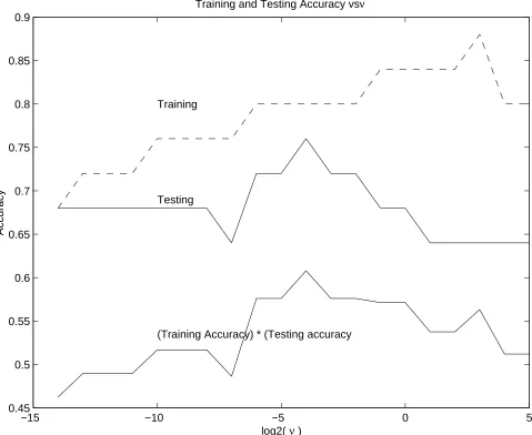
6.3 Training and testing accuracy vs. parameter . . . 52
6.4 Classification of galaxies from AGNs . . . 53
6.5 Plot of logarithm X-ray flux vs R band magnitude . . . 55
6.6 AGNs and galaxies separation via SVM . . . 56
List of Tables
3.1 Training cases . . . 17
5.1 Identified CHDF-N sources . . . 45
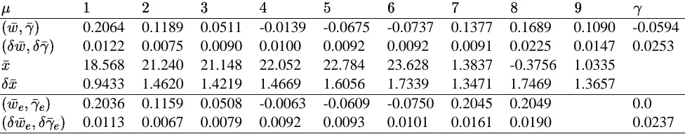
6.1 Separation plane parameters for star classification . . . 47
6.2 Plane parameters for AGNs and galaxies separation . . . 51
Chapter 1
Introduction
In real world environments that include data measurements in scientific research, a result may
be obtained with an upper limit value rather than a definite one. Even though a value is
ob-tained, it may contain significant errors. It becomes difficult or even impossible to improve
the quality of the data further because the result obtained has either reached the current
tech-nological limit in determining the accuracy of an attribute, or it has already been archived, or
improving it would be too costly. Technically, every numerical measurement contains some
er-rors. The problem to be addressed, therefore, is to determine if one can neglect the error. More
often than not, however, including data with upper and lower limits and errors may provide
more meaningful information or imply some constraints that would not be evident if the errors
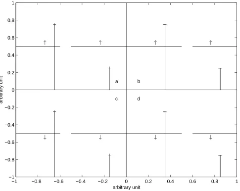
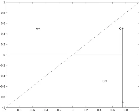
were dropped. In Fig. 1.1, a simple case is used to demonstrate the usefulness of including
these kinds of constraints.
respectively. For a binary class problem, +1 and -1 are convenient designations for their class
not only because of the sign discrimination, but also their fit into a formula for mathematical
treatment, as discussed in Chapter 8. Hereafter, +1 and -1 will be used as the binary classes
unless specifically stated otherwise. To classify them correctly, a separation plane is drawn as
the dash-dot line in Fig. 1.1 which satisfies their classifications. However, if there is another
data item which has an upper boundary on the vertical axis at C(3/4, 1/2) with class +1, then it
makes a difference whether one drops or includes it in determining the separation plane where
the vertical line below point C indicates that it is an upper limit with a boundary of 1/2 on its
vertical axis. In fact, the solid horizontal line separates the classes better than the dash-dot line
which misclassifies data C.
Data integration, or merge, may encounter different precision issues when more than one
of the primary databases do not match up properly in terms of accuracy. This phenomenon also
raises questions about precision. This integration trend can be expected to increase along with
the increase of accessing and processing databases via the Internet. Treatment of nonuniform
precision or hybrid data, therefore, needs to be addressed.
Many Machine Learning (ML) methods, from the simplest 1R rule [12] to more
sophisti-cated ones such as Support Vector Machines (SVMs [25]), recognize only data presumed to be
without any error or upper and lower limits. This limitation restricts the application of these
methods. Support Vector Machines (SVMs, [25]), representing one of the major kernel
meth-ods, are also powerful tools for data classification. A tutorial about SVMs can be found in
−1 −0.8 −0.6 −0.4 −0.2 0 0.2 0.4 0.6 0.8 1 −1
−0.8 −0.6 −0.4 −0.2 0 0.2 0.4 0.6 0.8 1
A
B
C
↓
8). This paper describes the linear SVMs developed in a domain that contains data with upper
or lower limits and data with error. As a comparison, Chapter 2 describes a possible scenario
with a 1R rule algorithm in such a domain. The treatment of this domain can be extended to
many other statistical based ML regimes, such as the Naive Bayes Network, Decision Tree, etc.
Treatments of such a domain are, however, quite different when using SVMs. Because of the
unique feature of the SVM separation plane to discriminate classes, one can derive a concise
mathematical formula to handle data conveniently in such a domain. A clean algorithm, based
on this concise formula, is possible to treat data in such a domain. This paper focuses on SVM
development in such domains in Chapters 3-6, which cover concepts, mathematical bases,
al-gorithms and application in a data set. These SVMs are called ULEDS-SVMs (Upper/Lower
Limit and Error Data Supported Support Vector Machines). The domains that contain data with
upper or lower limits and errors are called ULED domains. The advantage of ULEDS-SVMs
is obvious in terms of computing cost when comparing them to the enhanced 1R rule ML in a
ULED domain. In Chapter 3 some theorems which will be used as the basis for treating data
with upper or lower limits and data with errors in SVMs. Chapter 4 presents the generalized
algorithms of ULEDS-SVMs.
There are several databases which are regarded as benchmarks in the AI community for
algorithm testing and comparison, although none of these belongs to a ULED domain. Chapter
5 describes the integration of a data set from astronomical observations taken from Chandra
Deep Field (CDF) and Hubble Deep Field (HDF) North, or CDHF-N for short. The
These observations are focused on the sky direction which has the least galactic and
extragalac-tic obscuration and absorption. Long exposure times were devoted to image and spectroscopic
observations in various energy bands, including radio, infrared, optical and X-ray sources,
us-ing the largest telescopes on the ground as well as in outer space in order to understand the
dis-tribution and evolution of galaxies. This field contains many sources identified by their spectral
and morphological types. It also contains many unidentified sources whose further
identifica-tions are difficult, primarily because the instrument limits have been reached. In these sources,
some attributes contain only upper limits, but statistical study is nonetheless worthwhile given
the available data; other sources contain attributes which are relatively bright and saturated in
image observation. So, only the lower limit in terms of brightness was obtained. A data set,
CHDF-N, was generated from the sources collected from several literature sources and used as
the test bed. A review of the literature and a description of the effort made regarding the data
set integration are given in Chapter 5 and Appendix A. Chapter 6 and Appendix A describe the
source classification results for training, testing and prediction using ULEDS-SVMs.
Discus-sion and concluDiscus-sions are provided in Chapter 7. A general review of SVMs may be found in
Chapter 8. The code for the specific implementation of ULEDS Support Vector Machines is
Chapter 2
Enhanced 1R - A Simple Method to Treat
Data with Limit and Error Attributes
First, the definitions of upper and lower limits and of error are introduced. Such definitions help
to eliminate ambiguity about the meaning of these terms and help to establish the mathematical
foundation necessary to treat them.
Definition: Define
as a data set over variables or attributes. For a data point,
,
its th attribute,
, has an upper limit,
, only if the th attribute value, from its acquisition,
is unknown but less than the upper limit,
.
represents the upper limit along the th
component in
for the point.
An example of an upper limit of an attribute is found in the astronomical magnitude
mea-surement of objects. Within a given period of exposure time and using a specific telescope
is sufficiently bright. However, the object may be too faint to show up under such conditions.
When it cannot be detected, one can nevertheless derive a magnitude as the object brightness
limit, according to the observation specification and the background level of the direction. One
cannot know how much fainter the object would be than the limit magnitude; however, one
can say that the object is not brighter than the limit magnitude. Data with such an upper limit
attribute frequently appear, especially in scientific data measurement.
Similarly one can define the lower limits:
Definition: for a point,
, its th attribute,
, has a lower limit,
, only if the th
attribute,
. One refers to
as the lower limit on the th component in
for the
point.
Sometimes there could be an error obtained for a variable or attribute.
Definition: for a point,
, its th attribute,
, has an error,
#
, only if there
are both upper and lower limits on the th component such that
. When both
equalities hold, #
, the data do not have any errors on the th component. The value,
,
is called its centroid value of the th component of point
, and , of
’s lower and upper
limit on the th component, respectively.
is called the centroid point.
In the actual measurement of a quantity, the limit that is measured often refers to the limit
of at confidence level or some level. Error is often expressed as
at
confidence level or some level. Quite often a contour around the error or limit can also be
seen. This contour describes in terms of statistical uncertainty the limit value that is measured
the limits and errors. In most statistical learning processes, such a fine structure may not be
required; a representative sharp boundary for limits is sufficient in many cases. The most
frequent references to the confidence level of limits and errors are ,
,
or .
These are assumed to be true in the treatment of SVMs described in the following chapters;
however, the fine structure of the errors and limits will be touched on a little later in this
chapter for the enhanced 1R rule. More detailed statistical descriptions of errors and limits
may be found in textbooks about statistics and data reduction.
Here it is worth noting that the upper or lower limit is not a missing datum. For missing
data, one or more attributes are totally unknown. In contrast, the point with an upper or lower
limit does tell that the value along a component does not exceed or go below a certain value,
or
. Including upper or lower limit data usually provides more information than a missing
value would provide. Moreover, the constraint may be crucial to the support or elimination of
some models.
2.1
1R Rule Extension
There is a very simple classification rule, called 1R, provided by [12]. A simple algorithm is
implemented therein to treat data with limit and error attributes. This simple implementation
has two purposes: the first is to put into practice a statistical learning approach by treating data
with limits and errors; and second, it is to be used to compare the training approaches used here
with the more sophisticated SVM methods. The 1R rule predicts that the classes will all be the
somewhat oversimplified. But, according to [12], the 1R rule is efficient and has reasonably
good accuracy for most commonly used data sets. Details about its pseudocode can be found
in Appendix A of [12].
The 1R rule may now be extended to cases that contain data with an upper limit. Given
a point of data,
, in the attribute space,
,
, where is the class of
the item, assumes that the space is within the domain,
, where
the Greek subscript represents the attribute. If
has an upper limit along the th attribute
dimension, the probability of the
distribution is , where # (2.1)
for the attribute with the upper limit of data
. the probability for each element in the space
can be obtained, and the 1R rule can be determined by using the largest probability in the
space. For the case of the lower limit, the integration is over
.
In general, there is a probability,
, where # (2.2) where
are the attributes of the point,
, with upper or lower limits.
The three-dimensional integer matrix, $!"!$# % &
in [12], is the probability
inte-gration in space,
, at each corresponding element where is the class and
%
is the value
for the attribute,
&
described above into COUNT, an upper and lower limit case can be cast.
Data attributes with errors can be seen as the existence of data bound by both upper and
lower limits,
. Integration is performed within these boundaries. Thus, all 1R
rule algorithms of [12] can also be extended to data with error.
The probability distribution of the errors or the limits may not be known. Under such
circumstances, an empirical distribution of a constant probability,
# , is
assumed for one attribute upper limit case,
#
for a lower limit case, and
#
for an error attribute.
The error or limit box is used to obtain the probability,
# %
, when there is more
than one attribute involving errors or limits of a data point in space,
, where
%
rep-resents the volume of the box of the error or limits occupied in the space,
. There is a
probability of those data with limits or errors of
% & # %
to
be in the element of class, , with value,
%
, for the attribute,
&
, where
%
is the Volume of
an Element in%
in
.
The COUNTs of a class, , having a value, %
, for attribute, &
, is $!"!$# % &
for
data without any errors or limits. The final probability of data that include limits or errors is
$!"!$# % & # $!"!$# % &
% &
, where
is a weighting
parameter for limit and error.
#
corresponds to the equal weighting of limit or error data
with respect to data with definite values, while
#
corresponds to the dropping of all data
2.2
Comments
This simple treatment represents the current knowledge about data distribution in
space,
including both ordinary data with definite values and data with upper/lower limits and errors.
Wherever there is a data entity with specific values of attributes, it falls into the specific element
of the volume in
space. Wherever there is an error or limit, a probability exists and is
distributed somewhere in a volume box,
%
. Statistical learning based on this knowledge to
treat data, including upper/lower limit and error data, is resumed. The most likely occurrence
of the class throughout the training data set in 1R can thereby be obtained.
Alternatively, even without obtaining the most frequently occurring element class, the
frac-tional frequency of occurrence in the event space may be extended to some other statistical
learning methods based on probability distribution, such as the Naive Bayes network, Decision
Tree, clustering analysis, etc.
Calculating COUNT for ordinary data entities is straightforward. However, calculating
and and adding to COUNT may be computationally expensive because it must be
per-formed on each relevant element at a time. For a data point with limits or errors, the upper
boundary of the time complexity caused by adding its contribution to COUNT may extend
over the whole domain in . In cases where a large amount of data with limits and errors exists
and where these boundaries are not well constrained, special treatment of the addition process
is desirable in order to increase the speed. The acceleration algorithm may depend on the
dis-tribution of data within the database. Sparse data with limits and errors may use the algorithms
as a base, similar to the density probability technique. COUNT is then applied in addition to
#
. A drawback of such acceleration is the loss of the generality of the algorithms. The
next chapter focuses on SVM treatment, which is not extendable from the strategy proposed
in this section to treat limit and error data. However, the unique separation plane concept of
SVM treatment provides a basis for a concise mathematical expression to discriminate classes
Chapter 3
Mathematical Foundation for
ULEDS-SVMs
3.1
Training
According to conventional SVMs, a hyperplane divides two classes in a feature space so that
misclassification is minimized while the margin is maximized (see, e.g. [5]). This phenomenon
may be achieved, as shown in Figure 3.1, by optimizing the Lagrangian function,
s.t.
&
(3.1)
Here,
represents the normal to boundary planes of the support vectors,
#
, with
a separation plane,
#
; and
is the scalar relevant to the distance of the plane to the
coordinate system origin,
is the vector in
the classes in
, is the weighting parameter for the soft margin that serves to penalize
the mix at the specified level, is the ones vector, and the prime indicates the transpose of the
corresponding vector or matrix. The dual to a linear SVM is
& & s.t. # (3.2) where
is the vector for Lagrangian multipliers (see, e.g., [5]). By default, a two-class problem
has two classes dedicated as +1 and -1. The normal of the separation plane,
, is expected to
point to the +1 class side. A data item is represented as
, where is represented
by a vector for its attributes, and is a scalar for its class.
To introduce the upper or lower limit or an error in a data attribute and to obtain a
mathe-matical presentation of the treatment in such cases, the theorems below are introduced:
Theorem 1: An entity,
, with upper (lower) limits is necessary for consideration in
SVM training if and only if for every component, , among the components which contain
upper (lower) limits for
, the entity satisfies
(
for the lower limit),
where
is the th component of the separation plane normal, and is the sign of the class of
the entity.
This theorem is one of the bases of the algorithms to be developed here. It is proved for
the upper limit case only. Proof for the lower limit case is similar. According to
, four
configurations are possible, as shown in Table 3.1:
a) when
is positive and is also positive, the ”+1” class is expected to be above the plane
along the th component. But the point,
, has an upper limit,
−1 −0.8 −0.6 −0.4 −0.2 0 0.2 0.4 0.6 0.8 1 −1
−0.8 −0.6 −0.4 −0.2 0 0.2 0.4 0.6 0.8 1
↑ ↑ ↑ ↑
↓ ↓ ↓ ↓
−
−
−
−
a b
c d
arbitrary unit
arbitrary unit
−
−
−
−
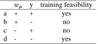
Figure 3.2: Four possible cases about and for upper limit shown in the four panels, a-d, corresponding to
Table . In each panel, the th component of the data, , may be above (left) or below (right) the separation
plane. Only in panels a and d does the position relevant to the separation plane make sense. The hypothetical separation plane is always satisfied in panels b and c no matter where the data item is positioned. The arrow in each figure points in a positive direction. The vertical line below the data + or - indicates that it is an upper
y training feasibility
a + + yes
b + - no
c - + no
d - - yes
Table 3.1: Training feasibility for the four cases of direction and class . See also Fig. a-d) for illustration.
sification if
was below the separation plane. That is to say, the separation plane does matter
in terms of classification in this case. In other words, the hypothesis that the plane predicts the
point correctly depends on the upper limit at the component,
. Therefore, training needs to
take this data into account;
b) when
is positive and is negative, the ”+1” class is expected to be above the separation
plane, and the ”-1” class below the separation plane along the th component. On the other
hand, this point has a negative class, and it has an upper limit along the th component. It does
not matter whether the upper limit point,
, is above the separation plane or not; the point
may not contradict the hypothetical classification according to the current separation plane. In
other words, one cannot reject the hypothesis that the plane correctly predicts the point class
anyway;
c) when
is negative and is positive, the ”+1” class is expected to be below the separation
plane along the th component. Wherever
is,
may not be above the plane, and
so the point may not contradict the separation that is expected with the prediction using the
separation plane along its th component. In other words, the hypothesis that the separation
plane correctly predicts the point class cannot be rejected;
d) when
plane, and the ”-1” class is expected to be above the separation plane.
is expected to be above
the plane. Because of the existence of the
upper limit, however, the point may or may not be
above the separation plane. Moreover, the point is absolutely below the separation plane when
is so. That is, the hypothesis that the separation plane correctly predicts the point class
depends on the upper limit,
. Classification training must take this point into consideration.
This generalization of the four cases provides the necessary and sufficient condition,
. Here, when the point falls on the plane, it is regarded as a positive classification; a parallel
plane along the axis means
#
. The parallel plane along the axis is not sensitive to
the location of
. So, the condition specified in Theorem 1 is also correct in both of these two
special cases. This completes the proof of Theorem 1.
Theorem 2: If a point, #
, containing upper (lower) limits satisfies the condition in
Theorem 1, its upper (lower) limit,
(
), of the th component can be used to replace
in
SVMs training.
Theorem 2 provides the basis for the iterative operation of the implementation of training
algorithms in ULEDS-SVMs. To prove the theorem, the upper limit case is considered. The
lower limit case can be similarly proved. Two cases need to be considered:
and # ; and and # . 1) and #
: First, it is necessary that every
of the point with a ”+1” class satisfies
the classification predicted correctly using the separation plane, if
can be so classified. It
also holds that if the plane misclassifies
, then it also misclassifies
. To prove this idea,
assume that
exists such that
is below the separation plane along its th component. Then, by definition,
must also be below the separation plane along the th component. So, using
to replace
is necessary. Second, it is sufficient to use
as the th component value to
replace
in training. To prove this, it is recognized that if a point at
is correctly classified,
it is above the separation plane along its component. This is an upper limit point. The
actual data point could be anywhere below this upper limit, but its exact location is unknown.
However, according to the definition of the hypothesis of plane separation, the hypothesis does
not contradict the classification of point,
, given the knowledge available.
2) By using a similar proof, it can be shown that
can replace
for the point when
and
#%
.
It can be proven that the lower limit,
, along every component can replace
in the lower
limit case. This completes the proof of Theorem 2.
Analogous to equations 3.1 and 3.2, the primal Lagrange function, including data with
upper and lower limits, is:
s.t. & (3.3)
and the dual to the Lagrange function can be written as:
&"& s.t. # (3.4)
diagonal matrix in
with diagonal elements. if for any upper limit or
if it is
for any lower limit component, and
#
otherwise. Here, corresponds
to the index of the item, while a Greek subscript corresponds to an attribute. The problem,
therefore, becomes a typical linear SVM problem. Available algorithms concerning SVMs are
applicable to treating data with upper and lower limit cases with such an embracement. They
can be adopted with the simple modification of keeping or dropping the entity with the upper
or lower limit under the conditions set forth in Theorem 1. If the entity is kept, it replaces the
corresponding value, according to Theorem 2.
In training, there are two possible approaches: training the whole data set with an mask,
as in the above equations, or training only the subset of the data which have the corresponding
non-zero mask value. The approach that is chosen will affect the time complexity and can be
determined by the fraction of the number of data entities with limits or errors (which will be
discussed later).
3.2
Test
According to Theorem 1, if
for an upper limit or
for a lower limit at any
attribute, , the classification is always correct. So, the test result is true. On the other hand, if
in the upper limit case or
in the lower limit case, according to Theorem 2, it
is necessary to test the upper (lower) limit point,
(
), against the separation plane in the same
way as one would if it had a definite value. That is, if
or
, then
test result is false.
First, this method utilizes the class, . And, it is applicable only for data with a limit case.
Alternatively, one can use the prediction method described in the next section and then
deter-mine if the prediction is the same as the given class. This utilizes the concept of predictability
(deferred to the next section). The current approach is nonetheless useful for the limit data test
because of the reduction in computing time.
3.3
Prediction
Unlike the use of conventional SVMs to predict definite data entities, predicting an entity with
an upper (lower) limit may result in ”+1”, ”-1” or ”unpredictable” which makes it impossible
to determine its class based on the uncertain attribute values if some conditions are satisfied.
Here, an intersection concept is introduced in order to cast the prediction feasibility.
Definition: for an upper (lower) limit case, if the upper (lower) limit point,
(
), is above
(below) the separation plane along its th component, then the actual entity value at the th
component,
, can be on either side of the separation plane. One says, then, that the upper
(lower) limit,
(
), intersects with the separation plane. If none of the upper (lower) limits
intersect with the plane, then one says that there is no intersection.
Extending the intersection concept further to data with error, one says that an entity has a
component with an intersection if both its upper and lower limits at the corresponding
compo-nent intersect with a separation plane.
the corresponding entity is not predictable. If an entity does not intersect with the separation
plane, then its class is predictable, and its class is as predicted for its upper (lower) limit point
for limit data or anywhere within the region of error for error data. A centroid value is chosen
in the error case.
For a compact expression of the next Theorem, the code,
!
, is denoted as a vector
of the limits, where ! #
represents the upper limit, -1 represents the lower limit and 0
represents the definite value of an attribute of the data,
, on the th component.
Theorem 3: The intersection and its inherent nonpredictability of a data point,
, is
determined by the existence of a component of such that # or !
for upper or lower limit data, and
for error data where
is the vector
of a data point,
the vector of the separation plane,
!
the code of limits on the th
component,
the vector of the point whose th component is set at its upper limit while the
other components are set at their centroid values, and
the vector of the point whose th
component is set at its lower limit while the other components are set at their centroid values.
This explanation leads to the proof of Theorem 3 from the geometric relationship of a data
point with limits or errors with respect to the separation plane. The condition of
#
indicates that the upper or lower limit is right at the separation plane. Since this is a limit point,
this means that it intersects with the plane. In the case where the actual data point falls on the
separation plane, one cannot tell to which class it belongs. So, it is appropriate that the data
point is included in the intersection case. In order to focus now on the other conditions, four
1)
, and indicate that the th component of the separation
plane normal points upward, and the limit point is above the separation plane along its th
component. But the point is an upper limit point, meaning that there is an intersection.
2) Similarly,
,
and
! #
indicate that the th component of the
plane normal points downward, and the limit point is below the separation plane along its th
component. But this point is a lower limit point, meaning that there is an intersection.
3)
and
and
! #
indicate that the th component of the plane normal
points upward, and the limit point is below the separation plane along its th component. But
this point is a lower limit point, meaning that there is an intersection.
4)
" ,
and
! #
indicate that the th component of the plane normal
points downward, and the limit point is above the separation plane along its th component.
But the point is an upper limit point, meaning that there is an intersection.
All four of these cases have exhausted the intersection cases where there is a limit in their
attributes. The combined formula satisfies
!
% . For error data, the following
case must be considered:
5)
means that the upper and lower boundaries are separated on either
side of the separation plane no matter which
direction the normal is, indicating that there is
an intersection. This proves Theorem 3.
With Theorems 1 and 3, one can immediately obtain:
Corollary: a datum with error is unpredictable if and only if it intersects with the separation
This is because if it intersects, one of the boundaries of the error must satisfy the Theorem 1
conditions. If it does not intersect, the boundaries of the error are on one side of the separation
plane.
It is worth pointing out that the feasibility for training addressed in Theorem 1 is different
from the feasibility of prediction addressed in Theorem 3 for limit cases. An item from a data
set may be trainable but not predictable, as shown, e.g., on the left plot in Fig. 3.2a. Similarly,
it may be predictable but not trainable, as shown, e.g., on the right plot in Fig. 3.2b. For data
with error, prediction feasibility leads to training feasibility and vice versa. This is because 1) if
the boundaries of an error along one attribute component are on the same side of the separation
plane in respect to this attribute, then there is no intersection. Training is feasible. 2) If both
boundaries of an error along one attribute component are on separate sides of the separation
plane in respect to this attribute, as expressed in the formula in Theorem 3 for error data, then
there is intersection. No matter what class the data item is in, and no matter what direction
goes, there is at least one boundary satisfying the Theorem 1 condition. Geometrically,
this point satisfies the hypothetical separation plane already, and it does not suggest any more
information about which way the separation plane would go during the current iteration for
Chapter 4
Algorithms
There are many implementations for SVMs, e.g., managing large data sets, such as
%
[15], based on [21]’s segmentation scheme, or addressing the issues for overcoming overfit,
such as the smooth method [18], etc. In chapter 8, a detailed review of the SVMs and some of
their recent developments is provided. The purpose of this section is not to provide a
bench-mark, but rather, discuss general algorithms which can be applied to the implementation of
most SVMs in domains that contain data with limits and errors, based on the principles
dis-cussed in the previous chapter.
First, the algorithms that handle data with upper and lower limits for training, testing and
prediction will be described. This idea is then extended to apply to data with errors. These
algorithms utilize available SVMs by invoking them directly in training; this is highly portable
from a software engineering point of view. Conventional SVMs do not need to be modified in
preparation of data by following the conditions that satisfy the trainability, as described above.
Then, the prepared data are fed to conventional SVMs for training.
When both limits and errors exist, the above scenario can also be used. However, with a
slight modification of conventional SVMs, the efficiency of the algorithms can be improved in
cases where a large fraction of limit or error data exists. This improvement can be achieved in
each iteration by preparing a mask for the data in order to satisfy the trainability conditions,
followed immediately by one iteration of the SVM training. An alternative approach may
also be considered to increase the SVM training iteration a few more steps, but this is not
necessary until the convergence of the computation process. Along with this approach, the
modification of conventional SVMs serves simply to reserve the Lagrangian multipliers from
the last iteration and use them as the initial Lagrangian multipliers in the next iteration. A
pseudocode sample for such a scenario is provided at the end of this chapter.
4.1
Upper and Lower Limit Case
4.1.1
Training
Let denote the set of all entities with the non-empty subset of which contains only
definite data and the subset of entities, , with upper or lower limits for at least one attribute
of each entity. Let
!
denote the set of code vectors of the attributes of the upper or lower limit
of each entity in , where 1 represents the upper limit, -1 represents the lower limit and 0
represents the definite value code. Let
#
entities and which contains untrainable entities with respect to a separation plane. Let a
working set
#
#
. And let
#
Algorithm 4.1.1: TRAINING( ) while do # # for each ! do if # ## # ! then # p else p # #
comment: invoke conventional training
# # if then # comment: #
, is the class of
4.1.2
Test
In addition to testing according to conventional methods, which do not have limits, one must
also consider the sign of
which differs from conventional testing. If the attribute of an
entity is for an upper limit or for a lower limit case, testing for this entity is always
true. Otherwise, it is the same as
to determine the correct classification. The
notation,
!
, as the code vector of the limit for an entity is used as the input parameter.
Algorithm 4.1.2: TEST(
)
comment:
- vector containing the attribute values for an entity
comment: - the class of the attribute
comment: - vector of entity attribute code: 1/-1/0 - upper/lower/no t limit
comment:
- separation plane direction and position vector/scalar
comment: RETURN - true for ”+1”, false for ”-1” class
4.1.3
Prediction
Predictability depends on whether the upper or lower limit point intersects with the separation
plane. The function of intersect, Lmt, utilizes Theorem 3. If there is no intersection, prediction
Algorithm 4.1.3: PREDICT(
)
comment:
- vector of entity attributes including limits
comment: - vector of entity attribute code: 1/-1/0 - upper/lower/no limit
comment:
- separation plane direction and position vector/scalar
comment: RETURN - class ”+1”, ”-1”, ”unpredictable”
if ## then else if then else if then # if # & ! then for each do if comment:
- th element of
4.2
Data With Error
4.2.1
Training
Similar to data with upper and lower limits, data with error can be treated the same as if both
upper and lower limits,
, are found along the same component. A hyper diamond box
formed by the limits surrounding the centroid value of the data point may intersect with the
hyperplane which separates the classes, or it may fall to one side of the plane. When there is
intersection, this data point is not trainable. Its classification is always true in testing. Because
it can be either class, it is nonpredictable. On the other hand, if there is no intersection, training,
testing and prediction may be undertaken in the same manner as using only the centroid value
of the data point. Conventional SVM algorithms are resumed using these values.
Here, the notation is extended into a space so as to cast the content of the centroid value,
the upper and lower boundaries, in case there is an error. Let denote the set of entities with
three-dimensional space,
. The first two dimensions are the same as the conventional
event matrix, but the third is an extension of its centroid value, the upper limit and lower limit
values of the corresponding event matrix. If data at an attribute have definite value, the centroid,
upper and lower limits are all equal to the definite value. If data at an attribute are at an upper
or lower limit, all three values are equal to the corresponding limit. A working set is in
. Further, the symbols,
and
, denote, as previously stated, an entity with attributes
that are all set at the centroid value, except along the th component which is set at its upper
function is not used. Rather, the predictability Err function is used.
Algorithm 4.2.1: TRAININGERR ( # ) while do # for each do if ## # ! then p
comment: invoke conventional training
4.2.2
Testing
When an entity is not predictable, there is an intersection between the hyper diamond error
box and the separation plane. This is set true in testing. Otherwise, the test is the same as that
performed at the centroid value of the hyper diamond error box. The algorithm is as follows:
Algorithm 4.2.2: TESTERR (
)
comment:
- the attribute of
comment: - the class of . is a short representation of
and
comment:
- separation plane normal and distance
if
## &
then else if then else
4.2.3
Predicting
Similarly, when a point has an error box that intersects with the hyperplane, it is unpredictable.
Otherwise, prediction is possible by using the attribute values of the centroid point with respect
Algorithm 4.2.3: PREDICTERR (
)
comment:
- the attributes of an entity
comment:
- separation plane normal and distance
if
# &
then else if then else
4.3
ULEDS-SVMs
The algorithms provided in the previous two sections treat data, including those with upper
and lower limits or with errors, respectively. When data have both limits and errors mixed
in the data set, the scenario used above can also be used. However, this section provides an
alternative algorithm to treat the training problem by masking out the untrainable items of data
and training the remaining entities within the same iteration loop. Next is the pseudocode for
this algorithm, ULEDS-SVMs. Here, the subsets are denoted as follows:
the set of data points with lower limits, definite values, and upper limits;
is the
set for the codes 1, -1, 0 and 2 that correspond to the upper limits, lower limits, error and
definite values, respectively;
is the set of classes of the items;
is the separation
plane; is the execution code for training, testing or prediction; and #
is the termination
condition. The
parameter in conventional SVMs is a vector for Lagrangian multipliers.
Modification of conventional SVMs can be restricted for output
after each convSVMTraining
iteration, and then input
as its initial parameter for training during the next iteration rather
than initiating
automatically within convSVMTraining. Iterate within convSVMTraining for
training only once or a few times; outside the convSVMTraining, use diag(mask)
to replace
the original
parameters. When there is both ”work” set stability and convSVMTraining
convergence, training stops at the separation plane,
Algorithm 4.3.1 - ULEDS-SVMs
ULEDS_SVMs(D, U, C, w, gamma, Op, Tcond)
// assert: D, U, C are in order of their corresponding attributes
init d_ret // common/static vector in Rˆn for attributes of one item m = size(C) // number of items in D
init d // init matrix for one item in D, with 3 frame
init u // init vector for one item in U
init c // init scalar for one item about class in Rˆ1
// branch according to Op - training, testing or predicting if Op == training // begin the training branch for ULED
init w,gamma
init mask // init mask vector,
init Work // init working set, as a subset of Rˆ{m n+1}
init iterT = false // init termination condition in iteration while iterT == false
Work = empty
// prepare the set by rejecting untrainable items in training for i <- 1:m
// extract one item from the dataset
(d, u, c) <- extract the ith items from (D, U, C)
// check out the trainability
if trainPredictability_ULED(d, u, c, w, gamma, Op) == true mask <- 1
else
mask <- 0
Work <- (d_ret, c) // item was put in the working set endfor
alpha = diag(mask) * alpha // mask out the non-trainable item
// invoke conventional SVMs training routine // with a little modification
call convSVMTraining(Work, w, gamma, alpha, Tcond)
if Work does not change in consequent iteration and Tcond satisfied iterT = true
endwhile
return -1 // return the -1 code after successful training
elseif Op == testing // begin testing branch
init Right // init the set in Rˆ{m n+1} classified correctly init Wrong // init the set in Rˆ{m n+1} classified incorrectly
for i <- 1:m // test the item one by one // extract one items from the dataset
(d, u, c) <- extract the ith items from (D, U, C)
// check if predictable or not
if trainPredictability_ULED(d, u, c, w, gamma, Op) == true // predictable, then test as for the normal predication case if c * (d_ret * w - gamma ) >= 0 // classified correctly
count++
Right <- (d_ret, c) // output into Right class set
else // misclassified
Wrong <- (d_ret, c) // output into Wrong class set else
// unpredictable, then set as classified right count++
Right <- (d_ret, c) // output into Right class set endfor
return count // return the correct classification number
elseif Op = predicting // begin predicting branch
for i <- 1:m // predict the items one by one
// extract one items from the dataset (d_class is unnecessary) (d, u, c) <- extract the ith items from (D, U, C)
if trainPredictability_ULED(d, u, c, w, gamma, Op) == true // predictable, then predict as definite case
if (d_ret * w - gamma ) > 0
Dclass(i) = 1 // +1 class
elseif (d_ret * w - gamma ) < 0
Dclass(i) = -1 // -1 class
elseif (d_ret * w - gamma ) = 0
Dclass(i) = 0 // right on separation plane
else
// unpredictable, then all set as 0 class C(i) = 0
endfor
function trainPredictability_ULED(d, u, c, w, gamma, Op)
// function for the trainability and predictability evaluation
n = size(u) // number of attributes
for mu <- 1:n
d_ret(mu) = d(mu,2) // assign the centroid value to d_ret endfor
for mu <- 1:n // loop run through the attributes
if u(mu) == 0
// case of attribute with error
if intersectCompErr(mu, d(mu,1), d(mu,3), w, gamma) == true return false
elseif abs(u(mu)) == 1
// case of attribute with limit (u(mu) = 1 or -1) if Op == training
if trainabilityCompLmt(u(mu), c, w(mu)) == false return false
if Op == testing or Op == predicting
if intersectCompLmt(mu, u(mu), w, gamma) == true return false
endfor return true
function intersectCompErr(mu, d_low, d_up, w, gamma)
xup <- d_ret // copy the vector for the centroid value into xup xup(mu) <- d_up // replace xup’s mu’th element by d_up
xlow <- d_ret // copy the vector for the centroid value into xlow xlow(mu) <- d_low // replace xup’s mu’th element by d_low
if (xup * w - gamma) * (xlow * w - gamma) <= 0
return true // one of theorem 3 intersection conditions satisfied else
return false // no intersection along this component
function intersectCompLmt(mu, u_mu, w, gamma)
f = d_ret * w - gamma // objective function
if f == 0 return true // one end of the limit right on the plane if f * w(mu) * u_mu > 0
return true // one of theorem 3 conditions satisfied
return false
function trainabilityCompLmt(u_mu, w_mu, c) if w_mu * u_mu * c <= 0
return false // theorem 1 condition violated
else
Chapter 5
Chandra and Hubble Deep Field North
(CHDF-N) dataset
Multiband observations for Hubble Deep Field (HDF) and Chandra Deep Field(CDF) North
are used as the test bed in this study. This sky direction is used to avoid, as much as possible, the
stars from our galaxy and interstellar media so that observations can be as deep as possible.
X-ray observations using Chandra are from [4]. This reference contains, in its original catalogue,
370 sources which were discovered using an average of about 1 Ms exposure observation. A
more recent result based on a 2 Ms exposure was also available [1] at the time this work was
completed. However, because the new catalogue contains a large fraction of the total sources
that contain observational results that are not publicly available at wavebands other than X-ray
for magnitudes similar to those used here, the 1 Ms catalogue is still used for this work. Three
the hard band, HB.
[2] provides a source catalogue with magnitudes at several energy bands other than the
X-ray band of [4]’s X-ray observations. The source attributes include the magnitudes from
submillimeter, 20 cm radio, infrared, and several optical filter photometric observations. The
20 cm radio survey observation contains a much less positive detection than upper limits. Even
though the method developed in this paper targets training with toleration regarding the
exis-tence of upper and lower limits and errors, this attribute was eliminated for the purpose of the
SVM training, testing and prediction. That is, in this research, the astronomical aspects of this
work are not emphasized. The field for submillimeter observations is much smaller than for
other observations. Therefore, there is a large number of missing values for the submillimeter
attribute. In addition, even within the observed area, there are many upper limits, or values with
large errors. So, here the submillimeter attribute is dropped, too, for the same reason that the
radio attribute was eliminated. The attributes now used include the infrared magnitude, HK’,
and optical magnitudes with filters of z’, I, R, V and B, with corresponding colors from red to
blue. The relationship between flux and magnitude is [?]
#
where
is the magnitude of an object, and
is the flux of the source. As defined, the brighter a
source, the less value its magnitude. So, for source saturation in a photometric observation, a
lower limit of its brightness may be obtained which corresponds to an upper limit in magnitude.
On the other hand, a faint source with a negative detection on some wavelengths results in an
upper limit of brightness which corresponds to a lower limit in magnitude. Magnitude limits
survey limits described in [2].
For classification of the objects, one of the most important methods is to categorize objects
into stars, galaxies, active galactic nuclei (AGNs), etc. The stars, galaxies and AGNs may
be further categorized according to subclasses. [13] identified and compiled, among 82 early
Chandra deep field X-ray sources, 32 sources for the classes of the objects. One of the sources,
(#39 in [13]), appears in neither [4]’s X-ray nor [2]’s optical catalogues. But, it is included
in [1]’s 2 Ms observation catalogue. Because there is a lack of attribute information for every
energy band except for X-rays, this source has been eliminated from the analysis.
Among the remaining 31 sources, there are 2 stars, 8 low luminous galaxies (LL), 7 high
luminous galaxies (HL), 8 broad line AGNs (BL), and 7 narrow line AGNs (NL). Given the
sample size of the identified objects, the low and high luminous galaxies are combined into
one class (-1), and the broad and narrow line AGNs into another (+1). Stars can be classified
relatively easily from multiband observations.
[2] also made spectroscopic observations of the bright optical counterparts of the 370 X-ray
sources. Although an atlas for the spectrum is provided, it has not been classified according
to the conventional types of astronomical objects, except for 5 stars. The intention here is
to integrate the data uniformly, and because the classification of stars is not a major issue of
astronomical interest here since the main focus is the classification of extragalactic objects, and
also because the classification for the known extragalactic objects is mainly in the subset that
does not interact with the star class, no further effort is made to include [2]’s stars in the data
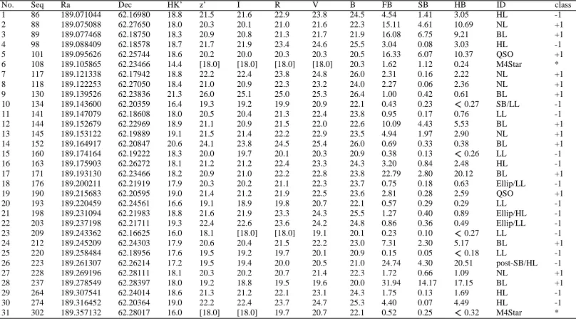
The composed data set for those objects with known identifications is shown in Table 5.1
with columns 1-2: the source sequence number in this Table and the source number in [4] [2];
columns 3-4: the source coordinates, Ra and Dec, from [2]. These coordinate attributes were
not used in training. Including these attributes here is for convenience of identification only;
columns 5-10: magnitudes of HK’, z’, I, R, V, and B from [2]; columns 11-13: X-ray flux in
a unit of ergs/cm
/s from [4]; columns 14-15: the source identification from [13] and
its digitized class, identified by combining galaxies as -1 and AGNs as +1, respectively, as
described above. The brackets ”[ ]” quote the upper limit of a magnitude where saturation was
encountered due to a bright source. This includes 2 stars (No. 6 & No. 31) and 1 galaxy (No.
23) at some optical wavelength with filter observations. In addition, 4 galaxies (No. 10, 15, 23,
25) have upper limits at the HB X-ray measurements, as marked by ” ”. Among these, source
No. 23 has both optical saturation and upper limits at the HB X-ray band.
It is reasonable to use a log scale for FB, SB and HB. But here in Table 5.1, the energy
flux is listed as the original linear scale, as in [4]. In the next chapter, it is log-scaled with
2.5*log(Flux) in training in order to scale up to match the scale in optical observations.
Without an identification constraint, there are 274 sources out of [4]’s original 370 sources
which satisfy the criteria. That is, the sources with the missing attributes were eliminated. This
information is compiled and presented in Table 9.1 in Appendix A where the values above the
slash indicate the magnitude and fluxes of the corresponding filter or energy bands, and the
values below the slash indicate the boundary code; this is a little different from
!
described in
No. Seq Ra Dec HK’ z’ I R V B FB SB HB ID class 1 86 189.071044 62.16980 18.8 21.5 21.6 22.9 23.8 24.5 4.54 1.41 3.05 HL -1 2 88 189.075088 62.27650 18.0 20.3 20.1 21.0 21.6 22.3 15.11 4.61 10.69 NL +1 3 89 189.077468 62.18750 18.3 20.9 20.8 21.3 21.7 21.9 16.08 6.75 9.21 BL +1 4 98 189.088409 62.18578 18.7 21.7 21.9 23.4 24.6 25.5 3.04 0.08 3.03 HL -1 5 101 189.095626 62.25744 18.6 20.2 20.0 20.3 20.3 20.5 16.33 6.07 10.37 QSO +1 6 108 189.105865 62.23466 14.4 [18.0] [18.0] [18.0] [18.0] 20.3 1.62 1.12 0.24 M4Star * 7 117 189.121338 62.17942 18.8 22.2 22.4 23.8 24.8 26.0 2.31 0.16 2.22 NL +1 8 118 189.122253 62.27050 18.4 21.0 20.9 22.3 23.2 24.0 2.27 0.06 2.36 NL +1 9 130 189.139526 62.23836 21.3 26.0 25.1 25.0 25.3 26.4 1.00 0.42 0.61 BL +1 10 134 189.143600 62.20359 16.4 19.3 19.2 19.9 20.9 22.1 0.43 0.23 0.27 SB/LL -1 11 141 189.147079 62.18608 18.0 20.5 20.4 21.3 22.4 23.8 0.95 0.17 0.76 LL -1 12 144 189.152679 62.22969 18.9 21.1 20.9 21.5 22.0 22.6 10.09 4.43 5.53 BL +1 13 145 189.153122 62.19889 19.1 21.5 21.4 22.2 22.9 23.5 4.94 1.97 2.90 NL +1 14 152 189.164917 62.20847 20.6 24.1 23.8 24.5 25.4 26.0 0.69 0.33 0.38 BL +1 15 160 189.174164 62.19222 18.3 20.0 19.7 20.1 20.3 20.9 0.38 0.13 0.26 LL -1 16 163 189.175903 62.26272 18.1 21.2 21.2 22.4 23.3 24.3 3.20 0.84 2.48 HL -1 17 171 189.193130 62.23466 18.2 20.9 21.0 22.2 22.8 23.8 22.79 2.80 20.12 BL +1 18 176 189.200211 62.21919 17.9 20.3 20.2 21.1 22.3 23.7 0.75 0.18 0.63 Ellip/LL -1 19 190 189.215683 62.20595 19.0 21.4 21.2 21.9 22.5 23.6 2.81 0.28 2.59 QSO +1 20 193 189.220459 62.24561 16.6 19.1 18.9 19.8 20.7 22.1 0.57 0.29 0.29 LL -1 21 198 189.231094 62.21983 18.8 21.6 21.9 23.3 24.3 25.5 1.27 0.40 0.89 Ellip/HL -1 22 203 189.237198 62.21711 19.3 22.4 22.6 23.6 24.2 24.8 0.86 0.36 0.49 Ellip/LL -1 23 209 189.243362 62.16625 16.0 18.1 [18.0] [18.0] 19.1 20.1 0.23 0.10 0.27 LL -1 24 212 189.245209 62.24303 17.9 20.6 20.4 21.5 22.2 23.0 7.31 2.30 5.17 BL +1 25 220 189.258484 62.18956 17.6 19.5 19.2 19.7 20.1 20.9 0.15 0.05 0.18 LL -1 26 223 189.261307 62.26214 17.2 19.5 19.4 20.0 20.5 21.0 24.74 4.30 20.51 post-SB/HL -1 27 228 189.269196 62.28111 18.1 20.3 20.2 20.7 21.4 22.3 1.72 0.66 1.09 NL +1 28 237 189.278549 62.28397 18.0 19.2 18.8 19.5 19.6 20.0 31.94 14.17 17.15 BL +1 29 264 189.307541 62.24014 18.6 21.3 21.2 22.1 23.1 24.3 1.75 0.13 1.69 HL -1 30 274 189.316452 62.20364 19.0 22.2 22.4 23.7 24.7 25.3 4.40 0.07 4.49 HL -1 31 302 189.357132 62.28017 16.0 [18.0] [18.0] 19.7 20.7 22.1 0.52 0.25 0.32 M4Star *
Table 5.1: Table of identified CHDF-N sources with identification for galaxies and AGNs. Two stars from
13
Chapter 6
Classification via ULEDS-SVM on
CHDF-N Dataset
6.1
Implementation of ULEDS-SVMs Incorporated with LSVM
Chapter 8 will provide a detailed review of the SVMs and their implementation. Many SVM
implementations exist that emphasize different aspects. For the purpose of an implementation
that extends SVMs into ULEDS-SVMs and applies these ULEDS-SVMs in the CHDF-N data
set, the Lagrangian SVM (LSVM) [20] was chosen as the conventional SVM that is most
relevant to ULEDS-SVMs. LSVM is simple in implementation within a Matlab environment
and is especially suitable to showcase in the classroom.
The code for ULEDS-SVMs used here is written in Matlab language to utilize the matrix
![Figure 3.1: Linear Separation Plane for the non-separable case.��� . Courtesy of [5]](https://thumb-us.123doks.com/thumbv2/123dok_us/1768400.1227542/25.595.131.451.225.485/figure-linear-separation-plane-non-separable-case-courtesy.webp)