Article
Structural Changes in Boreal Forests Can Be
Quantified Using Terrestrial Laser Scanning
Tuomas Yrttimaa 1,2*, Ville Luoma 2, Ninni Saarinen 2,1, Ville Kankare 1,2, Samuli Junttila 1,2, Markus Holopainen 2,3, Juha Hyyppä 3 and Mikko Vastaranta 1
1 School of Forest Sciences, University of Eastern Finland, Joensuu, 80101, Finland; [email protected]; [email protected]; [email protected];
2 Department of Forest Sciences, University of Helsinki, Helsinki, 00014, Finland; [email protected]; [email protected]; [email protected];
3 Department of Remote Sensing and Photogrammetry, Finnish Geospatial Research Institute, National Land Survey of Finland (NLS), Masala, 02431, Finland; [email protected];
* Correspondence: [email protected],; Tel.: +358-50-5127051
Received: date; Accepted: date; Published: date
Abstract: Terrestrial laser scanning (TLS) has been adopted as a feasible technique to digitize trees and forest stands, providing accurate information on tree and forest structural attributes. However, there is limited understanding on how a variety of forest structural changes can be quantified using TLS in boreal forest conditions. In this study, we assessed the accuracy and feasibility of TLS in quantifying changes in the structure of boreal forests. We collected TLS data and field reference from 37 sample plots in 2014 (T1) and 2019 (T2). Tree stems typically have planar, vertical, and cylindrical characteristics in a point cloud, and thus we applied surface normal filtering, point cloud clustering, and RANSAC-cylinder filtering to identify these geometries and to characterize trees and forest stands at both time points. The results strengthened the existing knowledge that TLS has the capacity to characterize trees and forest stands in space and showed that TLS could characterize structural changes in time in boreal forest conditions. Root-mean-square-errors (RMSEs) in the estimates for changes in the tree attributes were 0.99-1.22 cm for diameter at breast height (Δdbh), 44.14-55.49 cm2 for basal area (Δg), and 1.91-4.85 m for tree height (Δh). In general, tree attributes were estimated more accurately for Scots pine trees, followed by Norway spruce and broadleaved trees. At the forest stand level, an RMSE of 0.60-1.13 cm was recorded for changes in basal area-weighted mean diameter (ΔDg), 0.81-2.26 m for changes in basal area-weighted mean height (ΔHg), 1.40-2.34 m2/ha for changes in mean basal area (ΔG), and 74-193 n/ha for changes in the number of trees per hectare (ΔTPH). The plot-level accuracy was higher in Scots pine-dominated sample plots than in Norway spruce-dominated and mixed-species sample plots. TLS-derived tree and forest structural attributes at time points T1 and T2 differed significantly from each other (p < 0.05). If there was an increase or decrease in dbh, g, h, height of the crown base, crown ratio, Dg, Hg, or G recorded in the field, a similar outcome was achieved by using TLS. Our results provided new information on the feasibility of TLS for the purposes of forest ecosystem growth monitoring.
Keywords: spatiotemporal, time series, bi-temporal, ground-based LiDAR, tree growth
1. Introduction
Forests change over time and across space due to natural phenomena and anthropogenic processes. Biotic changes, such as forest growth and damage, affect forest structure and tree stems and branches grow annually in width and height. Conifer trees are typically evergreen but leaves of deciduous trees emerge in the spring and fall in the autumn. Forest growth process is also linked to the decomposition process which affects the amount of dead wood [1]. Insect damage, the spread of pathogens, wind damage, and forest fires, shape forests at different spatial and temporal scales. Insect damage, that is often combined with the spread of pathogenic fungi, causes defoliation and changes
in the bark whereas winds fall trees or cut tree parts [2] and fire burns low vegetation, needle mass and possibly also reshapes the structure of trees [3,4]. There are also abiotic changes that affect the forest structure. These include land-use changes as well as silvicultural and harvesting operations. In managed forests, trees are often planted, seedlings are tended, and several thinning operations are carried out during the rotation period [5]. Silvicultural practices vary a great deal, but in general, a proportion of trees is typically removed in silvicultural and harvesting operations [5,6]. Spatiotemporal information is needed to improve the understanding of, or quantify, the consequences of these natural phenomena, processes, and human activities with varying temporal and spatial patterns and dimensions.
Close-range sensing technologies, such as terrestrial laser scanning (TLS) provide state-of-the-art in characterizing forests. TLS is a powerful close-range sensing method for characterizing forests in three dimensions (3D; [1,7–10]). Individual trees can be detected from a TLS point cloud by detecting circular shapes (e.g. [11,12]) or clusters of points (e.g. [13,14]), these two representing the most common tree detection methods implemented in forest applications [8]. Then, depending on the algorithm used and the purpose of the processing, architectural structure of a stem [15,16] or a whole tree [17,18] can be reconstructed by using a series of geometrical primitives, preferably circular cylinders [19]. Tree reconstruction requires that points representing a tree are classified based on their origin, in other words from stem, branches, and foliage. Point cloud classification algorithms are most often based on an assumption that stem points have more planar, vertical and cylindrical characteristics than points originating from branches and foliage [10,15,17,20]. With careful TLS data collection and pre-processing, a single point in TLS data can reach a millimetre-level accuracy within the data set [21,22] meaning that the reconstructed tree models are geometrically highly accurate [18]. So far, there is a limited number of approaches for classifying points originating from foliage based on geometric features [23–26]. Use of radiometric features based on laser return intensity have been seen beneficial in separating foliage and woody material [27–29]. After tree architecture is reconstructed for every tree in an area of interest, theoretically all external tree dimensions can be derived from geometrically accurate 3D models for all trees and used further in deriving attributes of interest.
in stem forms. Of the 35 investigated trees, which were mainly conifers, changes in stem taper, cylindrical form factor, form quotient, and stem slenderness were analysed. The changes in the stem taper varied from -34% to 9%, the cylindrical form factor from 1% to 18%, the form quotient from 4% to 35%, and the stem slenderness from -2% to 6%.
The objective of this study was to strengthen the understanding how TLS can be used to capture boreal forest structure in space and time. Concentrating on the change of only a few attributes with a relatively low number of samples has been the common denominator for all the previous studies related to the use of TLS in quantifying changes in tree attributes. A more comprehensive investigation on the performance of capturing changes in tree and forest structural attributes with a large number of trees and sample plots is needed to assess the feasibility of TLS in monitoring forest structural changes. To fill in the knowledge gap, we used bi-temporal TLS data and field inventory data to cover changes in the structure of 1280 trees and 37 sample plots from varying boreal forest conditions. We hypothesized that TLS has the capacity to accurately estimate tree and forest structural attributes at single time points, and the estimated attributes at the beginning of a monitoring period significantly differ from the respective attributes at the end of the monitoring period. We assessed the performance of change quantification by using the most common tree and forest structural attributes. At tree level, we analysed changes in dbh (Δdbh), basal area (Δg), tree height (Δh), diameter-height ratio (Δd-h-ratio), height of the crown base (Δhc), and crown ratio (Δcr). At stand (sample plot) level, we analysed changes in basal-area weighted mean diameter (ΔDg) and - height (ΔHg), mean basal area (ΔG), and number of trees per hectare (ΔTPH). Thus, we used a range of attributes describing changes in horizontal and vertical forest structure.
2. Materials and Methods
2.1. Study materials
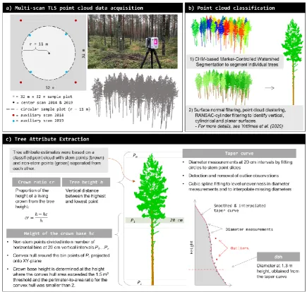
The study materials consisted of a multi-scan TLS data and a field inventory data acquired in 2014 (T1) and 2019 (T2) covering 1280 trees in 37 sample plots. The study site is located in Evo, southern Finland (61°19.6'N 25°10.8'E) where 91 sample plots (32 m x 32 m) were initially established in 2014 to cover the structural variation of forests (see e.g. [36]). A TLS data-acquisition campaign was carried out in spring 2014 using a Leica HDS6100 (Leica Geosystems, St. Gallen, Switzerland) and a Faro Focus 3D X330 (Faro Technologies Inc., Lake Mary, FL, USA) phase shift scanners, both operating at 1550 nm wavelength and measuring 508,000 points per second, delivering a hemispherical (310° vertical x 360° horizontal) point cloud with an angular resolution of 0.018° in both vertical and horizontal direction. A multi-scan approach was used to obtain a comprehensive point cloud for each sample plot by merging point clouds from five separate scanning locations. The scan setup consisted of one centre scan located at the plot centre and four auxiliary scans at quadrant directions (i.e. northeast, southeast, southwest, and northwest) about 11 m away from the plot centre. Artificial reference targets were used to register the point clouds together. Trees from each sample plot were located by manually detecting stem cross sections from horizontal TLS point cloud slices to construct a stem map. The stem maps were verified in the field and completed with the locations of small undergrowth trees that were not visible in the point cloud. A tree-wise field inventory was carried out in the summer of 2014 to acquire reference measurements of the tree attributes for T1. Tree species, dbh, h, hc, and health status (alive/dead) were recorded for all the trees with dbh exceeding 5 cm. Tree attributes were then aggregated at the plot level to obtain forest structural attributes: Dg (cm) and Hg (m), G (m2/ha), and TPH (n/ha). More detailed description on the TLS data acquisition and field inventory for T1 can be found in [22].
Switzerland) time-of-flight scanner that operates at 1550 nm wavelength and measures 2,000,000 points per second, delivering a hemispherical (300° vertical x 360° horizontal) point cloud with an angular resolution of 0.009° in both vertical and horizontal direction. Similar to T1 TLS data acquisition, a multi-scan approach (i.e. one centre scan with four auxiliary scans) was used in the T2 TLS campaign to ensure consistent point cloud quality. The scan setup for T2 was slightly modified from the one used in the T1 campaign based on experience gained in [10] that suggests placing the auxiliary scans approximately at the plot borders to improve point cloud completeness (see Figure 1). Artificial reference targets and a Leica Cyclone 3D Point Cloud Processing Software were used to register the separate point clouds together for each sample plot.
Later on, we found that, due to the slightly different scan setups used in the TLS-campaigns, the overall quality of the point clouds was somewhat poorer in T1 because the auxiliary scans in T1 were located closer to the plot center than in T2 (see Figure 1). Therefore the sample plots were reduced in size, from the rectangular 32 m x 32 m plots (1024.0 m2) to circular sample plots with a 11-m radius (380.1 m2), to achieve more comparable point clouds between time points T1 and T2 (i.e., to ensure that most of the trees were scanned from multiple directions). Thus, the total number of field-measured trees was 1280, of which 270 (21.1%) were Scots pine trees, 649 (50.7%) were Norway spruces (Picea abies (L.) H. Karst.), and 361 (28.2%) were broadleaved trees, mainly birches (Betula sp.) and European aspen (Populus tremula L.). The main tree species was defined for the sample plots based on proportional field-measured G at time point T2 by tree species. A sample plot was classified as a single species-dominated sample plot if any of the tree species accounted for more than 67% of the total basal area. Respectively, a sample plot was classified as a mixed-species sample plot if G of two or more tree species each accounted for more than 30% of the total basal area. This classification resulted in three groups of sample plots as 9 sample plots were classified as Scots pine-dominated, 13 sample plots were classified as Norway spruce-dominated, while 15 sample plots were classified as mixed-species sample plots. The sample plots covered a wide range of forest structural variation (see Table 1).
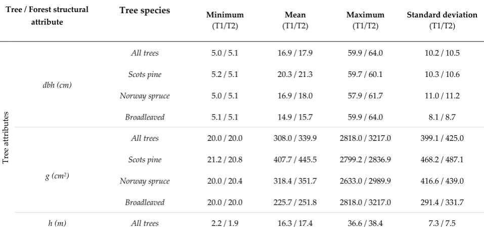
Table 1. Variation in tree attributes by tree species and forest structural attributes by main tree species of a sample plot, measured in 2014 (T1) and 2019 (T2). Diameter at breast height (dbh), basal area (g), tree height (h), diameter-height-ratio (d-h-ratio), height of the crown base (hc), and crown ratio (cr) were defined at tree level whereas basal area-weighted mean diameter (Dg) and - height (Hg), mean basal area (G), and number of trees per hectare (TPH) were defined at plot level. Scots pine-dominated plots = basal area of Scots pine (Pinus sylvestris L.) accounts for more than 67% of the total basal area of a plot. Norway spruce-dominated plots = basal area of Norway spruce (Picea abies (L.) H. Karst. ) trees accounts for more than 67% of the total basal area of a plot. Mixed-species plots = G of two or more tree species each account for more than 30% of the total basal area.
Tree / Forest structural attribute
Tree species Minimum
(T1/T2)
Mean (T1/T2)
Maximum (T1/T2)
Standard deviation (T1/T2)
Tr
ee a
tt
ri
bu
tes
dbh (cm)
All trees 5.0 / 5.1 16.9 / 17.9 59.9 / 64.0 10.2 / 10.5
Scots pine 5.2 / 5.1 20.3 / 21.3 59.7 / 60.1 10.3 / 10.6 Norway spruce 5.0 / 5.1 16.9 / 18.0 57.9 / 61.7 11.0 / 11.2
Broadleaved 5.1 / 5.1 14.9 / 15.7 59.9 / 64.0 8.1 / 8.7
g (cm2)
All trees 20.0 / 20.0 308.0 / 339.9 2818.0 / 3217.0 399.1 / 425.0
Scots pine 21.2 / 20.8 407.7 / 445.5 2799.2 / 2836.9 468.2 / 487.1
Scots pine 5.0 / 5.0 17.8 / 19.2 34.5 / 37.2 5.5 / 5.8
Norway spruce 2.2 / 3.5 15.2 / 16.4 36.6 / 38.4 8.4 / 8.5 Broadleaved 2.2 / 1.9 17.0 / 17.7 32.5 / 35.8 6.0 / 6.6
d-h-ratio
All trees 0.42 / 0.41 1.03 / 1.02 4.70 / 5.00 0.31 / 0.33
Scots pine 0.57 / 0.53 1.10 / 1.08 2.24 / 2.45 0.29 / 0.29
Norway spruce 0.73 / 0.65 1.09 / 1.08 2.86 / 2.15 0.21 / 0.19 Broadleaved 0.42 / 0.41 0.88 / 0.91 4.70 / 5.00 0.38 / 0.47 hc (m) Scots pine 4.2 / 6.3 12.2 / 13.9 23.1 / 24.6 3.4 / 3.4
cr Scots pine 0.22 / 0.19 0.40 / 0.37 0.69 / 0.59 0.09 / 0.08
F
o
res
t
str
u
ctu
ra
l
att
ri
bu
tes
Dg (cm)
All plots 13.0 / 14.3 27.5 / 28.8 42.8 / 44.0 9.3 / 9.3
Scots pine-dominated 14.2 / 15.1 21.7 / 22.9 30.6 / 31.7 4.5 / 4.5 Norway spruce-dominated 19.7 / 21.2 34.8 / 36.1 42.8 / 44.0 6.9 / 6.9
Mixed-species 13.0 / 14.3 24.8 / 26.2 42.8 / 43.2 9.7 / 9.7
Hg (m)
All plots 12.4 / 13.7 22.3 / 23.6 31.6 / 32.4 4.9 / 4.9
Scots pine-dominated 12.4 / 13.7 18.4 /20.0 23.1 / 25.3 3.2 / 3.4
Norway spruce-dominated 18.4 / 20.3 26.9 / 28.2 31.6 / 32.4 3.6 / 3.7 Mixed-species 15.9 / 17.3 20.8 / 21.9 27.3 / 27.8 3.6 / 3.5 All plots 15.3 / 17.2 31.6 / 34.5 51.5 / 56.8 10.5 / 11.0
G (m2/ha) Scots pine-dominated 15.3 / 17.2 22.6 / 25.5 31.1 / 34.4 5.9 / 6.8
Norway spruce-dominated 21.3 / 23.7 37.6 / 39.9 51.0 / 53.8 8.7 / 8.9 Mixed-species 16.2 / 17.5 32.4 / 35.9 51.5 / 56.8 10.6 / 11.7
TPH (n/ha)
All plots 368 / 368 1059 / 1045 3341 / 3236 706 / 711
Scots pine-dominated 368 / 368 963 / 997 1894 / 2105 495 / 553
Norway spruce-dominated 395 / 368 635 / 605 1289 / 1289 289 / 301
Mixed-species 526 / 552 1522 / 1488 3341 / 3236 847 / 835
2.2. Deriving tree and forest structural attributes from point clouds
distinguished by applying surface normal filtering, point cloud clustering, and Random Sample Consensus (RANSAC)-cylinder filtering on horizontal point cloud slices. A more detailed description of the point cloud classification procedure can be found in [37].
Figure 1. Outline of the TLS data processing workflow. One center scan and four auxiliary scans were used to acquire a multi-scan TLS point cloud data in 2014 and 2019 (a). TLS-based canopy height model (CHM) and a Marker-Controlled Watershed Segmentation procedure was applied to TLS point clouds to detect individual trees. Surface normal filtering, point cloud clustering and Random Sample Consensus (RANSAC)-based cylinder filtering were applied to identify vertical, cylindrical, and planar surfaces to classify TLS point cloud into stem and non-stem points (for more details, see [37]) (b). Then, the classified point cloud was used to extract tree attributes, namely diameter-at-breast-height (dbh) and tree diameter-at-breast-height (h) for all the trees, and diameter-at-breast-height of the crown base (hc) and crown ratio (cr) for Scots pine (Pinus sylvestris L.) trees (c).
missing diameters as suggested in [40]. Dbh was then obtained as the diameter at 1.3 m height from the taper curve. Tree-level g was computed from dbh measurements by considering the stem cross section as a circle (g = π * dbh2 / 4) and d-h-ratio was computed as a ratio between dbh and h (d-h-ratio = dbh / h). Hc was determined by first binning the non-stem points into horizontal slices with a height of 20 cm, then computing a convex hull around the bin points projected to XY-plane and hc was determined at the height where the convex hull area exceeded a 1.5 m2 threshold and the perimeter-to-area ratio for the convex hull was smaller than 2 (Figure 1c). Cr was computed as the proportion of the height of a living crown from the tree height (cr = (h - hc) / h). Finally, the forest structural attributes (i.e. Dg, Hg, G, and TPH) were computed by aggregating the tree-level attributes at the plot level (Table 2). Dg and Hg were computed as a basal area-weighted mean from the TLS-derived dbh and h measurements whereas G was a sum of g and TPH was the total number of trees within a sample plot per unit area.
Table 2. Description of the attributes used in this study to characterize trees and forest structure in 2014 (T1) and 2019 (T2). A = sample plot area in hectares, n = number of trees within a sample plot.
Tree / forest structural attribute Abbreviation Description / formula
Tr
ee
at
tr
ib
ut
es
diameter-at-breast-height (cm) dbh tree diameter measured at a 1.3-m height
basal area (cm2) g
π * dbh2 / 4
tree height (m) h vertical distance between ground and treetop
diameter-height ratio d-h-ratio dbh / h
height of the crown base (m) hc height of the lowest living branches
crown ratio cr (h - hc) / h
F
or
es
t
st
ruc
tura
l
at
tr
ib
ut
es
basal area-weighted mean diameter (cm) Dg ∑ 𝑑𝑏ℎ𝑖∗ 𝑔𝑖
𝑛
𝑖=1
/ ∑ 𝑔𝑖 𝑛
𝑖=1
basal area-weighted mean height (m) Hg ∑ ℎ𝑖∗ 𝑔𝑖
𝑛
𝑖=1
/ ∑ 𝑔𝑖 𝑛
𝑖=1
mean basal area (m2/ha) G ∑ 𝑔
𝑖 𝑛
𝑖=1
/ 𝐴
number of trees per hectare (n/ha) TPH n / A
2.3. Quantifying changes in tree and forest structural attributes
d-h-ratio (Δd-h-d-h-ratio), hc (Δhc) and cr (Δcr). At plot level, we analysed changes in TPH (ΔTPH), G (ΔG), Dg (ΔDg), and Hg (ΔHg).
2.4. Assessing the performance of the TLS-based method in quantifying changes in forest structure
Performance of the TLS-based method to quantify changes in tree attributes and forest structure was assessed by comparing the TLS point cloud-derived tree and forest structural attributes with the field-measured counterparts. For each TLS-derived tree, a corresponding field-measured tree was searched based on its spatial location. Capability of the TLS-based method to detect trees from the point clouds was then assessed by using completeness as an accuracy measure, indicating how large a part of the trees was detected from the point clouds. Accuracy of the TLS point cloud-derived estimates for tree and forest structural attributes at time points T1 and T2 as well as their difference (Δ) was assessed by using bias (mean error) and root-mean-square-error (RMSE) as accuracy measures:
𝑏𝑖𝑎𝑠 = ∑ (𝑋̂ − 𝑋𝑖 𝑖)
𝑛 𝑖=1
𝑛
(1)
𝑅𝑀𝑆𝐸 = √∑ (𝑋̂ − 𝑋𝑖 𝑖)
𝑛 𝑖=1
2
𝑛
(2)
where n is the number of trees or sample plots, 𝑋̂i is the TLS point cloud-derived tree attribute or forest structural attribute for tree or plot i, and Xi is the corresponding attribute based on reference measurements. Relative RMSE (RMSE%) and bias (bias%) were computed by dividing the absolute RMSE and bias with average value of the respective field-measured attribute. For tree attributes, the accuracy was assessed by tree species (Scots pine, Norway spruce, and broadleaved trees) while for forest structural attributes the accuracy was assessed by main tree species of a sample plot (Scots pine-dominated, Norway spruce-dominated, and mixed-species sample plots). Coefficient of determination (R2) was used to measure the relationship between the TLS point cloud-derived and field-measured tree and forest structural attributes. Paired-sample T-tests were used to test whether the TLS-based estimates for tree and forest structural attributes at time point T1 significantly differed from the respective estimates at time point T2.
3. Results
3.1. Performance of detecting trees using bi-temporal TLS data
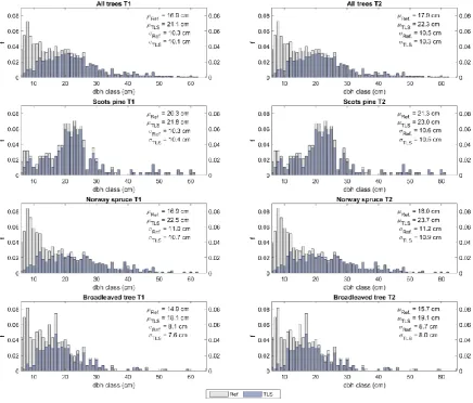
Out of the total number of 1280 trees that were measured in the field, 795 trees (62.1%) were detected from the point clouds at both timepoints T1 and T2. The detected trees represented 84.5% of the total basal area of all trees. Tree detection accuracy was highest among Scots pine trees, followed by Norway spruce and broadleaved trees (Table 3). Trees that remained undetected were mainly small in size, while large trees were detected at both timepoints with high accuracy (Figure 2).
Table 3. The number of trees by tree species that were measured in the field (Nref) and detected from the TLS point clouds (NTLS) at the beginning (2014) and at the end of the monitoring period (2019). Completeness indicates how large a part of the detected trees represented the total number and the total basal area of the field measured trees.
Tree species Nref NTLS Completeness:
total stem number
Completeness: total basal area
All trees 1280 795 62.1% 84.5%
Scots pine 270 227 84.1% 91.3%
Norway spruce 649 366 56.4% 85.7%
Figure 2. Diameter at breast height (dbh) distributions presenting the relative frequency (f) of trees in 1 cm dbh classes by tree species. Mean values (μ) and standard deviations (σ) based on field (Ref) and terrestrial laser scanning (TLS) measurements are presented as well. The coloured bars represent the proportion of trees by dbh classes that were detected from the TLS point clouds at both timepoints 2014 (T1) and 2019 (T2).
3.2. Performance of characterizing trees in space using TLS
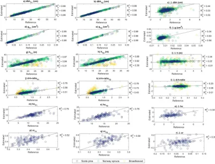
Strong relationships (R2 = 0.99) between the field-measured and TLS-derived estimates for dbh and g were recorded at both timepoints (Figure 3a-b, 3d-e). Dbh was estimated with an RMSE of 1.18 cm (5.7%) and 0.90 cm (4.1%) at T1 and T2, respectively, with no significant (p > 0.05) differences in accuracy between the tree species (Table 4). However, g was estimated more accurately for Norway spruce (RMSE% 6.2-10.6%) than for Scots pine (RMSE% 12.5-13.0%) and broadleaved trees (RMSE% 14.5-16.0%). On average, dbh of Norway spruce were overestimated by 0.26-0.30 cm, while dbh of Scots pine and broadleaved trees were underestimated by 0.43-0.32 cm and 0.03-0.19 cm, respectively. Considering all the trees, slightly lower RMSEs and biases of dbh and g were obtained at T2 than at T1.
species. R2 of 0.76-0.79 was recorded between the field-measured and TLS-derived d-h-ratio for Scots pine, while the respective values for Norway spruce and broadleaved trees were 0.58-0.73 and 0.43-0.51, respectively (Figure 3j-k).
Hc and cr were estimated for Scots pine trees only. R2 between the field-measured and TLS-derived estimates for hc and cr were 0.78-0.79 and 0.52-0.58, respectively (Figure 3p-q). For hc estimates an RMSE of 2.71 m (25.7%) for T1 and 2.55 m (20.4%) for T2 with an underestimate of 1.36-1.70 m (Table 4). On average, cr was overestimated by 10.3-11.7% with a relative RMSE of 22.5-22.8% (Table 4).
Figure 3. Relationship between the field-measured reference measurements and the TLS-derived estimates on tree attributes, such as diameter-at-breast-height (dbh), basal area (g), tree height (h), diameter-height-ratio (d-h-ratio), and crown ratio (cr) by tree species measured in 2014 (T1) and 2019 (T2) as well as their difference (Δdbh, Δg, Δh, Δd-h-ratio, and Δcr). The solid black line represents the 1:1 relationship between the reference and the estimated values. R2p, R2s, and R2b denote coefficient of determination for Scots pine, Norway spruce, and broadleaved trees, respectively.
Table 4. Bias and root-mean-square-error (RMSE) of TLS-derived estimates for tree attributes, namely diameter-at-breast-height (dbh), basal area (g), tree height (h), diameter-height-ratio (d-h-ratio), height of the crown base (hc) and crown ratio (cr) by tree species at time points T1 (2014) and T2 (2019) as well as their change (Δ). Negative bias denotes underestimation.
Tree
Attribute Tree species
Bias RMSE
T1 T2 Δ T1 T2 Δ
dbh (cm)
All trees -0.05 (-0.3%) 0.04 (0.2%) 0.10 (8.3%) 1.18 (5.7%) 0.90 (4.1%) 1.13 (97.4%)
Scots pine -0.43 (-2.0%) -0.32 (-1.4%) 0.12 (10.1%) 1.11 (5.2%) 0.99 (4.5%) 0.99 (83.9%)
Broadleaved -0.19 (-1.1%) -0.03 (-0.15%) 0.17 (15.0%) 1.11 (6.3%) 0.99 (5.27%) 1.12 (100.4%)
g (cm2)
All trees -7.65 (-1.9%) -3.39 (-0.7%) 4.26 (10.2%) 49.28 (11.9%) 47.59 (10.4%) 49.40 (118.4%)
Scots pine -21.47 (-5.1%) -18.48 (-3.9%) 2.99 (7.0%) 52.82 (12.5%) 60.81 (13.0%) 44.14 (102.8%)
Norway spruce 1.75 (0.4%) 7.38 (1.4%) 5.64 (12.9%) 50.51 (10.6%) 32.35 (6.2%) 55.49 (126.6%)
Broadleaved -9.16 (-3.1%) -5.96 (-1.8%) 3.21 (8.7%) 42.42 (14.5%) 53.51 (16.3%) 42.98 (117.1%)
h (m)
All trees -1.33 (-6.9%) -0.74 (-3.6%) 0.59 (42.1%) 4.37 (22.5%) 4.10 (19.7%) 3.53 (251.6%)
Scots pine -0.89 (-4.8%) -0.47 (-2.3%) 0.43 (27.3%) 2.52 (13.7%) 2.42 (12.1%) 1.91 (122.8%)
Norway spruce -0.51 (-2.6%) 0.39 (1.8%) 0.90 (72.3%) 3.99 (20.1%) 3.03 (14.4%) 3.43 (274.6%)
Broadleaved -3.31 (-16.8%) -3.11 (-14.6%) 0.21 (13.8%) 6.26 (31.7%) 6.56 (30.8%) 4.85 (321.5%)
d-h-ratio
All trees 0.10 (9.7%) 0.07 (6.3%) -0.04 (226.6%) 0.35 (33.6%) 0.30 (29.5%) 0.33 (2028.6%)
Scots pine 0.05 (4.6%) 0.03 (2.6%) -0.02 (78.3%) 0.28 (24.9%) 0.24 (21.6%) 0.28 (942.6%)
Norway spruce 0.06 (5.3%) -0.01 (0.1%) -0.06 (563.8%) 0.26 (23.6%) 0.16 (14.8%) 0.22 (2123.3%)
Broadleaved 0.24 (26.9%) 0.23 (26.2%) -0.01 (88.6%) 0.53 (59.8%) 0.51 (57.7%) 0.49 (4516.2%)
hc (m) Scots pine -1.70 (-16.1%) -1.36 (-10.9%) 0.34 (20.7%) 2.71 (25.7%) 2.55 (20.4%) 1.97 (120.6%)
cr Scots pine 0.05 (11.7%) 0.04 (10.3%) -0.01 (36.2%) 0.10 (22.8%) 0.09 (22.5%) 0.09 (318.1%)
3.2. Performance of characterizing tree attributes in time using TLS
It was possible to quantify changes in tree attributes using TLS. Paired sample T-tests showed that the tree attributes estimated at T1 significantly (p < 0.01) differed from the respective attributes estimated at T2 (Table 5). Relationship between the changes in field-measured and TLS-derived tree attributes was stronger for attributes characterizing changes in horizontal tree structure (i.e., Δdbh and Δg) than attributes characterizing changes in vertical tree structure (i.e., Δh, Δhc, and Δcr; Figure 3). In general, the changes in tree attributes were estimated with smaller RMSE for Scots pine than for Norway spruce and broadleaved trees (Table 4). RMSE in Δdbh estimates was 0.99-1.22 cm (83.9-103.5%), and most often Δdbh was overestimated by 0.04-0.17 cm (3.8-15.0%) depending on tree species. Differences in the accuracy of Δg estimates between the tree species were small and not considered statistically significant (p > 0.05). On average, Δh was overestimated by 0.21-0.90 m (13.8-72.3%) with an RMSE of 1.91-4.85 m (122.8-321.5%). In this case, the highest accuracy was recorded for Scots pine, followed by Norway spruce and broadleaved trees. The accuracy of Δd-h-ratio was considerably lower than the accuracy of other tree attributes. Relative errors in Δd-h-ratio were large (RMSE 942.6-4516.2%) due to uncertainty in tree height estimates.
Attributes characterizing changes in crown structure were estimated for Scots pine trees only. With TLS, 34% and 35% of the variation in Δhc and Δcr respectively, was possible to capture. On average, Δhc was overestimated by 0.34 m (20.7%) with an RMSE of 1.97 m (120.6%) which is at the same level to the accuracy of Δh estimates for Scots pine trees (Table 4). Relative errors in Δcr estimates were larger (RMSE% 318.1%) due to uncertainty in h and hc estimates.
Table 5. The p-values from the paired-sample T-tests indicating the significance of the differences between the TLS-derived estimates of tree attributes, such as diameter-at-breast-height (dbh), basal area (g), tree height (h), diameter-height-ratio (d-h-ratio) and crown ratio (cr) by tree species measured in 2014 (T1) and 2019 (T2).
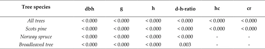
Tree species dbh g h d-h-ratio hc cr
All trees < 0.000 < 0.000 < 0.000 < 0.000 < 0.000 < 0.000 Scots pine < 0.000 < 0.000 < 0.000 < 0.000 < 0.000 < 0.000 Norway spruce < 0.000 < 0.000 < 0.000 < 0.000 - -
3.3. Performance of characterizing forest structural attributes in space with TLS
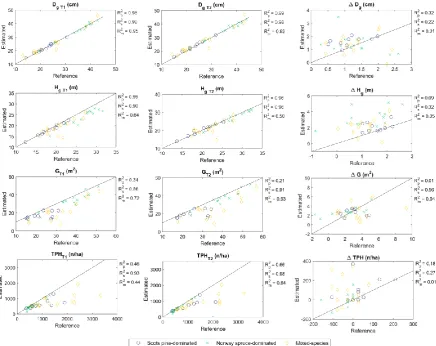
Forest structural attributes were estimated accurately with TLS point clouds from the both timepoints. Strong relationships (R2 > 0.86) between the field-measured and the TLS-derived estimates for Dg, Hg, G, and TPH were recorded for Norway spruce-dominated sample plots (Figure 4). On Scots pine-dominated sample plots, the R2 indicated stronger relationship between the field-measured and the point cloud-derived estimates for Dg and Hg (R2 > 0.96) than for TPH (R2 = 0.46-0.66) and G (R2 = 0.21-0.34). On mixed-species sample plots, an R2 of 0.93-0.95 was recorded for Dg, 0.50-0.64 for Hg, 0.63-0.72 for G, and 0.44-0.63 for TPH. Considering all the sample plots, the estimation accuracy for Dg and G was at the same level for T1 and T2 while Hg and TPH estimates seemed to be slightly more accurate at T2 (RMSE% 7.9% for Hg and 49.3% for TPH) than at T1 (RMSE% 11.2% for Hg and 58.5% for TPH; Table 6).
Dg was underestimated by 0.15-0.26 cm (0.4-0.7%) on Norway spruce-dominated sample plots while overestimated by 0.08-0.55 cm (0.4-2.4%) on Scots pine-dominated, and by 0.39-0.41 cm (1.6%) on mixed-species sample plots (Table 6). More accurate estimates for Dg were recorded on Norway spruce-dominated and Scots pine-dominated sample plots (RMSE% 2.5-3.4%) than on mixed-species sample plots (RMSE% 8.4-9.6%). Hg was underestimated on all the sample plots by 0.35-2.88 m (1.9-10.7%) except Scots pine-dominated plots at T2 when it was overestimated by 0.20 m (1.0%). Accuracy of Hg estimates was highest on Scots pine-dominated sample plots (relative RMSE 2.9-3.5%) followed by Norway spruce-dominated (RMSE% 3.9-11.6%) and mixed-species sample plots (RMSE% 12.6-13.1%).
Figure 4. Relationship between the field-measured reference measurements and the TLS-derived estimates on forest structural attributes, such as basal area-weighted mean diameter (Dg) and -height (Hg), mean basal area (G), and number of trees per hectare (TPH) by main tree species in 2014 (T1) and 2019 (T2) as well as their difference (ΔDg, ΔHg, ΔG, and ΔTPH). The solid black line represents the 1:1 relationship between the reference and the estimated values. R2p, R2s, and R2b denote coefficient of determination for Scots pine-dominated, Norway spruce-dominated, and mixed-species forest plots, respectively.
Table 6. Bias and root-mean-square-error (RMSE) of TLS-derived estimates for forest structural attributes, namely basal area-weighted mean diameter (Dg) and - height (Hg), mean basal area (G) and number of trees per hectare (TPH) in 2014 (T1) and 2019 (T2) as well as their change (Δ). Negative bias denotes underestimation.
Forest structural Attribute
Main tree species
Bias RMSE
T1 T2 Δ T1 T2 Δ
Dg (cm)
All plots 0.08 (0.3%) 0.25 (0.9%) 0.17 (13.2%) 1.42 (5.2%) 1.72 (6.0%) 0.93 (72.6%)
Scots pine-dominated 0.08 (0.4%) 0.55 (2.4%) 0.47 (40.5%) 0.59 (2.7%) 0.77 (3.4%) 0.60 (52.5%)
Norway
spruce-dominated -0.26 (-0.7%) -0.15 (-0.4%) 0.10 (7.8%) 0.87 (2.5%) 1.06 (2.9%) 1.13 (86.4%) Mixed-species 0.39 (1.6%) 0.41 (1.6%) 0.02 (1.4%) 2.09 (8.4%) 2.51 (9.6%) 0.91 (67.9%)
Hg (m)
All plots -1.73 (-7.8%) -0.50 (-2.1%) 1.24 (96.3%) 2.51 (11.2%) 1.85 (7.9%) 1.64 (127.8%)
Scots pine-dominated -0.35 (-1.9%) 0.20 (1.0%) 0.55 (35.3%) 0.53 (2.9%) 0.70 (3.5%) 0.81 (51.9%)
Norway
Mixed-species -1.67 (-8.0%) -0.69 (-3.1%) 0.98 (86.6%) 2.72 (13.1%) 2.76 (12.6%) 1.39 (122.9%)
G (m2/ha)
All plots -6.49 (-20.5%) -6.60 (19.1%) -0.11 (-3.7%) 8.52 (26.9%) 9.27 (26.9%) 1.84 (64.2%)
Scots pine-dominated -5.32 (-23.6%) -5.56 (-21.8%) -0.23 (-8.1%) 7.03 (31.1%) 8.05 (31.6%) 1.40 (48.9%)
Norway
spruce-dominated -3.84 (-10.2%) -3.24 (-8.1%) 0.59 (26.4%) 5.09 (13.5%) 4.23 (10.6%) 1.48 (66.4%) Mixed-species -9.79 (-30.2%) -10.46 (-29.2%) -0.67 (-19.3%) 11.50 (35.5%) 12.82 (35.7%) 2.34 (68.0%)
TPH (n/ha)
All plots -373 (-35.2%) -292 (-27.9%) -81 (-570%) 620 (58.5%) 515 (49.3%) 143 (1008.7%)
Scots pine-dominated -337 (-35.0%) -268 (-26.9%) -68 (-200.0%) 486 (50.5%) 428 (42.9%) 130 (381.5%)
Norway
spruce-dominated -91 (-14.3%) -47 (-7.7%) -45 (-146.7%) 117 (18.5%) 65 (10.7%) 74 (245.1%) Mixed-species -659 (-43.3%) -536 (-36.0) -124 (-366.7%) 914 (60.0%) 753 (50.6%) 193 (569.3%)
3.4. Performance of characterizing forest structural attributes in time using TLS
Changes in forest structural attributes were quantified using TLS. Paired sample T-tests showed that Dg, Hg, and G estimated at T1 significantly (p < 0.000) differed from the respective attributes estimated at T2 (Table 7). In case of TPH the differences between T1 and T2 estimates were not considered significant (p > 0.05). Based on field measurements, TPHT1 was significantly larger than TPHT2 on Norway spruce-dominated and mixed-species sample plots due to fallen or harvested trees. On these sample plots, some of the trees that were fallen or harvested were not detected at T1 and thus, change in TPH was not captured. On Scots pine-dominated sample plots, however, the change in TPHwas not considered significant and thus, not expected to be captured with TLS. In general, accuracy of characterizing changes in forest structural attributes was at a higher level on Scots pine-dominated sample plots than on Norway spruce-pine-dominated and mixed-species sample plots (Table 6).
Relationship between the field-measured and TLS-derived estimates for ΔDg were similar on Scots pine-dominated and Norway spruce-dominated sample plots (R2 of 0.32 and 0.22, respectively) while being considerably lower on mixed-species sample plots (R2 = 0.01, Figure 4). On average, ΔDg was overestimated by 0.02-0.47 cm (1.4-40.5%, Table 6). Most accurate estimates for ΔDg were obtained on Scots pine-dominated sample plots (RMSE% 52.5%) followed by mixed-species sample plots (RMSE% 67.9%) and Norway spruce-dominated sample plots (RMSE% 86.4%).
In case of ΔHg, the relationship between the field-measured and the TLS-derived estimates was the strongest on Norway spruce-dominated sample plots (R2 = 0.32) while being considerably lower on Scots pine-dominated and mixed-species sample plots (R2 = 0.05-0.09). On average, ΔHg was overestimated by 0.55 m (35.3%), 2.05 m (165.0%), and 0.98 m (86.6%) with an RMSE of 0.81 m (51.9%), 2.26 m (182.2%), and 1.39 m (122.9%) on Scots pine-dominated, Norway spruce-dominated and mixed-species sample plots, respectively (Table 6).
R2 indicated a considerably stronger relationship between the field-measured and the TLS-derived estimates for ΔG on Norway spruce-dominated sample plots (R2 = 0.56) than on Scots pine-dominated and mixed-species sample plots (R2 = 0.01-0.04). On Norway spruce-dominated sample plots, ΔG was overestimated by 0.59 m2/ha (26.4%) while on Scots pine-dominated and mixed-species sample plots ΔG was underestimated by 0.23 m2/ha (8.1%) and 0.67 m2/ha (19.3%), respectively (Table 6). The estimation accuracy was the highest on Scots pine-dominated sample plots (RMSE% 48.9%) followed by Norway spruce-dominated and mixed-species sample plots (RMSE% 66.4-68.0%).
Relationship between the field-measured and the TLS-derived estimates for ΔTPH was the strongest on Norway spruce-dominated sample plots (R2 = 0.27) followed by Scots pine-dominated sample plots (R2 = 0.18, Figure 4). On average, ΔTPH was underestimated on all the sample plots by 45-124 n/ha (146.7-366.7%). The highest accuracy of ΔTPH estimates was obtained on Norway spruce-dominated sample plots (RMSE% 245.1%) followed by Scots pine-spruce-dominated sample plots (RMSE% 381.5%) and mixed-species sample plots (RMSE% 569.3%).
Table 7. The p-values from the paired-sample T-tests indicating the significance of the differences between the TLS-derived estimates on forest structural attributes, such as basal area-weighted mean diameter (Dg) and - height (Hg), mean basal area (G) and trees per hectare (TPH) by main tree species measured in 2014 (T1) and 2019 (T2).
Main tree species Dg Hg G TPH
All plots < 0.000 < 0.000 < 0.000 0.105
Scots pine-dominated < 0.000 < 0.000 < 0.000 0.014
Norway spruce-dominated < 0.000 < 0.000 < 0.000 0.775
Mixed-species < 0.000 < 0.000 < 0.000 0.984
4. Discussion
The objective of this study was to assess the feasibility of TLS in characterizing boreal forest structure in space and time. We used a bi-temporal TLS dataset covering a five-year growth period in between the data acquisition campaigns in 2014 (T1) and 2019 (T2) and analysed the accuracy of the TLS-based method to quantify changes in tree and forest structural attributes. The results showed that changes in tree and forest structural attributes were captured using TLS. In general, tree and forest structural attributes estimated at T1 differed significantly (p < 0.01) from the respective estimates at T2 (Tables 5, 7). Only in case of TPH the differences in the TLS-derivedestimates at T1 and T2 were not considered statistically significant due to incomplete tree detection. In general, changes in the tree attributes were estimated more accurately for Scots pine trees, followed by Norway spruce and broadleaved trees (Table 4). Similarly, the accuracy of characterizing changes in forest structural attributes was higher on Scots pine-dominated sample plots than on Norway spruce-dominated and mixed-species sample plots (Table 6).
Vertical point cloud occlusion causes uncertainty in h estimates as dense canopy layers and overlapping crowns block the visibility from a scanner to treetops [8,46]. Thus, performance of TLS-based approaches to correctly estimate h has been identified as a major bottleneck hindering the use of TLS in practical forest inventory applications [47]. This was confirmed also in this study, as h was underestimated due to limited visibility to treetops. An RMSE of 4.10-4.37 m (19.7-22.5%) in h estimates was recorded for all the trees which is in line with previous findings in comparable forest conditions [43,47]. As expected based on results reported in [41], accuracy of characterizing forest height was improved at the sample plot level where an RMSE of 1.85-2.51 m (7.9-11.2%) was recorded for Hg estimates. For Scots pine trees, hc was successfully estimated by investigating the outer dimensions of a horizontally binned point cloud consisting of non-stem points (see Figure 1). Accuracy in hc estimates was similar to h estimates of Scots pine trees, providing reliable estimates for cr (Table 4).
The absolute errors in quantifying changes in tree attributes were, in general, at the same level than the errors in characterizing the attributes at T1 and T2 (Table 4). However, the bi-temporal TLS data used in this study covered only five growing seasons, which is a very short time when considering the lifetime of Scots pine or Norway spruce trees normally reaching the age from 80 to 120 years in boreal forests. Thus, changes in tree and forest structural attributes were relatively small, which explains why the errors in quantifying changes in tree attributes were rather large relative to the field-measured changes. In this study, for example, RMSE in dbh estimates (0.90-1.18 cm) was similar to the recorded average increase in dbh (1.16 cm). Short monitoring periods have been still applied in the previous studies related to investigating changes in forest structure using TLS due to the novelty of the method. In this case, it needs to be noted that the effect of measurement errors play an important role when the changes in the monitored attributes were small. This means that, for example, the recorded changes in dbh and h can be within the expected errors of both TLS-based and traditional measurement methods reported by [8,48]. As Luoma et al. [48] showed earlier, there is some variation also in the calliper and clinometer measurements when the measurements are repeated, which can depend on the different measurement positions (e.g. determining the breast height for dbh measurements) among other subjective factors. Dendrometers, such as a girth band for tree diameter measurement [49], provide probably the most accurate observations for monitoring changes in the dimensions of a living tree. However, dendrometers only measure one attribute at a time (e.g. dbh) and installing girth bands on a large number of trees to only monitor changes in dbh at forest stand level is rather expensive. Thus, data from clinometer and calliper measurements is typically used as a reference for tree attributes. But with their reliability being on a similar level to TLS-derived estimates, especially when measuring tree stem diameters, it needs to be remembered that actually either one of the measurements could be the ground truth, or the true value may be somewhere between the two observations. With longer monitoring periods, changes in tree attributes are expected to be larger and thus, the effect of the measurement errors should decrease, which further improve the reliability of change monitoring. Despite the variation in accuracies, the results of this study allow us to expect that with longer time periods, also the relative accuracies in change monitoring will be improved when the changes in tree attributes to be captured also increases..
The results of this study confirm the feasibility of TLS in characterizing forest structure in space and time. If an increase or decrease in tree and forest attributes was recorded in the field with conventional mensuration tools, a similar outcome was achieved by using bi-temporal TLS data. TPH was the only attribute that could not be characterized in time due to incomplete tree detection at both timepoints. Changes in TPH were minor, mostly because of a couple of fallen or harvested trees per sample plot during the monitoring period. Thus, it is evident that all trees should be characterized at the beginning and at the end of the monitoring period to reliably estimate ΔTPH. This requires better performance in tree detection which could be achieved with a more complete coverage of TLS data to avoid horizontal point cloud occlusion. However, increasing the number of individual scans used in a multi-scan approach decreases the cost-efficiency of TLS data acquisition. Use of mobile laser scanning (MLS) instead, where a point cloud is collected with a laser scanner mounted on an all-terrain vehicle [50,51] or a backpack [51,52], or with a hand-held laser scanner [53,54], would presumably be a more cost-efficient option to cover entire forest stands. When combined with SLAM (Simultaneous Localization and Mapping) -technology [55], the accuracy of MLS-derived tree attribute estimates is expected to be close to the TLS-derived estimates [52,54]. Another mobile platform for a laser scanner to suit close-range forest monitoring is an unmanned aerial vehicle (UAV) which can be used to collect detailed point clouds from above a forest canopy [56–58]. Due to different data acquisition geometries between terrestrial and UAV-borne point clouds, UAV-borne laser scanning is more suitable for characterization of the vertical forest structure whereas TLS or MLS can better capture the horizontal forest structure. An alternative option to combine the benefits of both terrestrial and aerial point cloud-based approaches is to collect the UAV-borne point clouds from inside the canopy [59] or to use a multisensorial approach [60] where photogrammetric UAV point clouds were integrated with TLS data. Use of a combination of bi-temporal terrestrial and aerial point clouds is expected to improve the accuracy of vertical forest characterization in space and time.
5. Conclusions
It is known that TLS is capable of characterizing forest structure in detail in space. Thus far, there has been a limited understanding on how forest structural changes can be quantified using TLS in time in boreal forest conditions. The results of this study confirm the capacity of TLS in providing information on the changes in tree and forest structural attributes. If an increase or decrease in tree and forest attributes was recorded in the field with callipers and clinometers, a similar outcome was achieved by using bi-temporal TLS data. However, incomplete digitization of trees and forest stands due to vertical and horizontal occlusion causes uncertainty in TLS-derived estimates in tree and forest attributes and their changes. Vertical occlusion could be decreased by using a combination of terrestrial and aerial point cloud data. Horizontal occlusion could be decreased with more complete point clouds by applying MLS technique to preserve cost-efficiency in data acquisition.
In this study, changes in tree and forest structural attributes were small due to a relatively short monitoring period. It is expected that, with a longer monitoring time the changes in tree attributes become more reliably detectable when automated point cloud-based approaches are used in boreal forest conditions.
Author Contributions: Conceptualization, M.V., N.S., V.K., T.Y., and V.L.; methodology, T.Y., V.K., N.S.; formal analysis, T.Y.; investigation, T.Y. and V.L.; resources, M.V., M.H., and J.H.; writing—original draft preparation, T.Y., V.L., S.J., N.S. and M.V.; writing—review and editing, all authors; supervision, N.S. and M.V..; project administration, M.V.; funding acquisition, M.V. and M.H. All authors have read and agreed to the published version of the manuscript.
Funding: This research was funded by Academy of Finland, grant numbers 272195, 307362, 331711.
Acknowledgments: The authors would like to thank Häme University of Applied Sciences for supporting the research activities in Evo.
References
1. Yrttimaa, T.; Saarinen, N.; Luoma, V.; Tanhuanpää, T.; Kankare, V.; Liang, X.; Hyyppä, J.; Holopainen, M.; Vastaranta, M. Detecting and characterizing downed dead wood using terrestrial laser scanning. ISPRS J. Photogramm. Remote Sens.2019, 151, 76–90.
2. Saarinen, N.; Vastaranta, M.; Honkavaara, E.; Wulder, M.A.; White, J.C.; Litkey, P.; Holopainen, M.; Hyyppä, J. Using multi-source data to map and model the predisposition of forests to wind disturbance. Scandinavian Journal of Forest Research 2016, 31, 66–79.
3. Carvajal-Ramírez, F.; da Silva, J.R.M.; Agüera-Vega, F.; Martínez-Carricondo, P.; Serrano, J.; Moral, F.J. Evaluation of Fire Severity Indices Based on Pre- and Post-Fire Multispectral Imagery Sensed from UAV. Remote Sensing 2019, 11, 993.
4. Gupta, V.; Reinke, K.; Jones, S.; Wallace, L.; Holden, L. Assessing Metrics for Estimating Fire Induced Change in the Forest Understorey Structure Using Terrestrial Laser Scanning. Remote Sensing 2015, 7, 8180–8201.
5. Holopainen, M.; Vastaranta, M.; Hyyppä, J. Outlook for the Next Generation’s Precision Forestry in Finland. Forests 2014, 5, 1682–1694.
6. Liang, X.; Hyyppä, J.; Kaartinen, H.; Holopainen, M.; Melkas, T. Detecting Changes in Forest Structure over Time with Bi-Temporal Terrestrial Laser Scanning Data. ISPRS International Journal of Geo-Information 2012, 1, 242–255.
7. Dassot, M.; Constant, T.; Fournier, M. The use of terrestrial LiDAR technology in forest science: application fields, benefits and challenges. Annals of Forest Science 2011, 68, 959–974.
8. Liang, X.; Kankare, V.; Hyyppä, J.; Wang, Y.; Kukko, A.; Haggrén, H.; Yu, X.; Kaartinen, H.; Jaakkola, A.; Guan, F.; et al. Terrestrial laser scanning in forest inventories. ISPRS Journal of Photogrammetry and Remote Sensing 2016, 115, 63–77.
9. Newnham, G.J.; Armston, J.D.; Calders, K.; Disney, M.I.; Lovell, J.L.; Schaaf, C.B.; Strahler, A.H.; Mark Danson, F. Terrestrial Laser Scanning for Plot-Scale Forest Measurement. Current Forestry Reports 2015, 1, 239–251.
10. Yrttimaa, T.; Saarinen, N.; Kankare, V.; Liang, X.; Hyyppä, J.; Holopainen, M.; Vastaranta, M. Investigating the Feasibility of Multi-Scan Terrestrial Laser Scanning to Characterize Tree Communities in Southern Boreal Forests. Remote Sensing 2019, 11, 1423.
11. Maas, H. ‐G; ‐G. Maas, H.; Bienert, A.; Scheller, S.; Keane, E. Automatic forest inventory parameter determination from terrestrial laser scanner data. International Journal of Remote Sensing 2008, 29, 1579– 1593.
12. Aschoff, T.; Thies, M.; Spiecker, H. Describing forest stands using terrestrial laser-scanning. International Archives of Photogrammetry, Remote Sensing and Spatial Information Sciences2004, 35, 237–241.
13. Cabo, C.; Ordóñez, C.; López-Sánchez, C.A.; Armesto, J. Automatic dendrometry: Tree detection, tree height and diameter estimation using terrestrial laser scanning. International Journal of Applied Earth Observation and Geoinformation 2018, 69, 164–174.
14. Zhang, W.; Wan, P.; Wang, T.; Cai, S.; Chen, Y.; Jin, X.; Yan, G. A Novel Approach for the Detection of Standing Tree Stems from Plot-Level Terrestrial Laser Scanning Data. Remote Sensing 2019, 11, 211. 15. Liang, X.; Litkey, P.; Hyyppa, J.; Kaartinen, H.; Vastaranta, M.; Holopainen, M. Automatic Stem Mapping
Using Single-Scan Terrestrial Laser Scanning. IEEE Transactions on Geoscience and Remote Sensing 2012, 50, 661–670.
16. Heinzel, J.; Huber, M. Detecting Tree Stems from Volumetric TLS Data in Forest Environments with Rich Understory. Remote Sensing 2016, 9, 9.
17. Raumonen, P.; Kaasalainen, M.; Å kerblom, M.; Kaasalainen, S.; Kaartinen, H.; Vastaranta, M.; Holopainen, M.; Disney, M.; Lewis, P. Fast Automatic Precision Tree Models from Terrestrial Laser Scanner Data. Remote Sensing 2013, 5, 491–520.
18. Hackenberg, J.; Morhart, C.; Sheppard, J.; Spiecker, H.; Disney, M. Highly Accurate Tree Models Derived from Terrestrial Laser Scan Data: A Method Description. Forests 2014, 5, 1069–1105.
19. Å kerblom, M.; Raumonen, P.; Kaasalainen, M.; Casella, E. Analysis of Geometric Primitives in Quantitative Structure Models of Tree Stems. Remote Sensing 2015, 7, 4581–4603.
20. Olofsson, K.; Holmgren, J. Single Tree Stem Profile Detection Using Terrestrial Laser Scanner Data, Flatness Saliency Features and Curvature Properties. Forests 2016, 7, 207.
21. Wilkes, P.; Lau, A.; Disney, M.; Calders, K.; Burt, A.; de Tanago, J.G.; Bartholomeus, H.; Brede, B.; Herold, M. Data acquisition considerations for Terrestrial Laser Scanning of forest plots. Remote Sensing of Environment 2017, 196, 140–153.
forest inventories. ISPRS Journal of Photogrammetry and Remote Sensing 2018, 144, 137–179.
23. Moorthy, S.M.K.; Krishna Moorthy, S.M.; Calders, K.; Vicari, M.B.; Verbeeck, H. Improved Supervised Learning-Based Approach for Leaf and Wood Classification From LiDAR Point Clouds of Forests. IEEE Transactions on Geoscience and Remote Sensing 2020, 58, 3057–3070.
24. Å kerblom, M.; Raumonen, P.; Casella, E.; Disney, M.I.; Danson, F.M.; Gaulton, R.; Schofield, L.A.;
Kaasalainen, M. Non-intersecting leaf insertion algorithm for tree structure models. Interface Focus2018, 8, 20170045.
25. Vicari, M.B.; Disney, M.; Wilkes, P.; Burt, A.; Calders, K.; Woodgate, W. Leaf and wood classification framework for terrestrial LiDAR point clouds. Methods in Ecology and Evolution 2019, 10, 680–694. 26. Ma, L.; Zheng, G.; Eitel, J.U.H.; Monika Moskal, L.; He, W.; Huang, H. Improved Salient Feature-Based
Approach for Automatically Separating Photosynthetic and Nonphotosynthetic Components Within Terrestrial Lidar Point Cloud Data of Forest Canopies. IEEE Transactions on Geoscience and Remote Sensing 2016, 54, 679–696.
27. Béland, M.; Baldocchi, D.D.; Widlowski, J.-L.; Fournier, R.A.; Verstraete, M.M. On seeing the wood from the leaves and the role of voxel size in determining leaf area distribution of forests with terrestrial LiDAR. Agricultural and Forest Meteorology 2014, 184, 82–97.
28. Zhu, X.; Skidmore, A.K.; Darvishzadeh, R.; Olaf Niemann, K.; Liu, J.; Shi, Y.; Wang, T. Foliar and woody materials discriminated using terrestrial LiDAR in a mixed natural forest. International Journal of Applied Earth Observation and Geoinformation 2018, 64, 43–50.
29. Junttila, S.; Holopainen, M.; Vastaranta, M.; Lyytikäinen-Saarenmaa, P.; Kaartinen, H.; Hyyppä, J.; Hyyppä, H. The potential of dual-wavelength terrestrial lidar in early detection of Ips typographus (L.) infestation – Leaf water content as a proxy. Remote Sensing of Environment 2019, 231, 111264.
30. Srinivasan, S.; Popescu, S.C.; Eriksson, M.; Sheridan, R.D.; Ku, N.-W. Multi-temporal terrestrial laser scanning for modeling tree biomass change. Forest Ecology and Management 2014, 318, 304–317.
31. Kaasalainen, S.; Krooks, A.; Liski, J.; Raumonen, P.; Kaartinen, H.; Kaasalainen, M.; Puttonen, E.; Anttila, K.; Mäkipää, R. Change Detection of Tree Biomass with Terrestrial Laser Scanning and Quantitative Structure Modelling. Remote Sensing 2014, 6, 3906–3922.
32. Sheppard, J.; Morhart, C.; Hackenberg, J.; Spiecker, H. Terrestrial laser scanning as a tool for assessing tree growth. iForest - Biogeosciences and Forestry 2017, 10, 172–179.
33. Hess, C.; Härdtle, W.; Kunz, M.; Fichtner, A.; von Oheimb, G. A high-resolution approach for the spatiotemporal analysis of forest canopy space using terrestrial laser scanning data. Ecol. Evol.2018, 8, 6800–6811.
34. Kunz, M.; Fichtner, A.; Härdtle, W.; Raumonen, P.; Bruelheide, H.; von Oheimb, G. Neighbour species richness and local structural variability modulate aboveground allocation patterns and crown morphology of individual trees. Ecol. Lett.2019, 22, 2130–2140.
35. Luoma, V.; Saarinen, N.; Kankare, V.; Tanhuanpää, T.; Kaartinen, H.; Kukko, A.; Holopainen, M.; Hyyppä, J.; Vastaranta, M. Examining Changes in Stem Taper and Volume Growth with Two-Date 3D Point Clouds. Forests 2019, 10, 382.
36. Vastaranta, M.; Yrttimaa, T.; Saarinen, N.; Yu, X.; Karjalainen, M.; Nurminen, K.; Karila, K.; Kankare, V.; Luoma, V.; Pyörälä, J.; et al. Airborne laser scanning outperforms the alternative 3D techniques in
capturing variation in tree height and forest density in southern boreal forests. Baltic For.2018, 28, 268–277. 37. Yrttimaa, T.; Saarinen, N.; Kankare, V.; Hynynen, J.; Huuskonen, S.; Holopainen, M.; Hyyppä, J.;
Vastaranta, M. Performance of terrestrial laser scanning to characterize managed Scots pine (Pinus sylvestris L.) stands is dependent on forest structural variation 2020.
38. Popescu, S.C.; Wynne, R.H. Seeing the Trees in the Forest. Photogrammetric Engineering & Remote Sensing 2004, 70, 589–604.
39. Meyer, F.; Beucher, S. Morphological segmentation. Journal of Visual Communication and Image Representation 1990, 1, 21–46.
40. Saarinen, N.; Kankare, V.; Vastaranta, M.; Luoma, V.; Pyörälä, J.; Tanhuanpää, T.; Liang, X.; Kaartinen, H.; Kukko, A.; Jaakkola, A.; et al. Feasibility of Terrestrial laser scanning for collecting stem volume
information from single trees. ISPRS Journal of Photogrammetry and Remote Sensing 2017, 123, 140–158. 41. Yrttimaa, T.; Saarinen, N.; Kankare, V.; Liang, X.; Hyyppä, J.; Holopainen, M.; Vastaranta, M. Investigating
the Feasibility of Multi-Scan Terrestrial Laser Scanning to Characterize Tree Communities in Southern Boreal Forests. Remote Sensing 2019, 11, 1423.
42. Abegg, M.; Kükenbrink, D.; Zell, J.; Schaepman, M.E.; Morsdorf, F. Terrestrial Laser Scanning for Forest Inventories—Tree Diameter Distribution and Scanner Location Impact on Occlusion. For. Trees Livelihoods 2017, 8, 184.
forest inventories. ISPRS Journal of Photogrammetry and Remote Sensing 2018, 144, 137–179.
44. Gollob, C.; Ritter, T.; Wassermann, C.; Nothdurft, A. Influence of Scanner Position and Plot Size on the Accuracy of Tree Detection and Diameter Estimation Using Terrestrial Laser Scanning on Forest Inventory Plots. Remote Sensing2019, 11, 1602.
45. Trochta, J.; Král, K.; Janík, D.; Adam, D. Arrangement of terrestrial laser scanner positions for area-wide stem mapping of natural forests. Canadian Journal of Forest Research 2013, 43, 355–363.
46. Schneider, F.D.; Kükenbrink, D.; Schaepman, M.E.; Schimel, D.S.; Morsdorf, F. Quantifying 3D structure and occlusion in dense tropical and temperate forests using close-range LiDAR. Agricultural and Forest Meteorology 2019, 268, 249–257.
47. Wang, Y.; Lehtomäki, M.; Liang, X.; Pyörälä, J.; Kukko, A.; Jaakkola, A.; Liu, J.; Feng, Z.; Chen, R.; Hyyppä, J. Is field-measured tree height as reliable as believed – A comparison study of tree height estimates from field measurement, airborne laser scanning and terrestrial laser scanning in a boreal forest. ISPRS Journal of Photogrammetry and Remote Sensing 2019, 147, 132–145.
48. Luoma, V.; Saarinen, N.; Wulder, M.; White, J.; Vastaranta, M.; Holopainen, M.; Hyyppä, J. Assessing Precision in Conventional Field Measurements of Individual Tree Attributes. Forests 2017, 8, 38. 49. Pesonen, E. A new girth band for measuring stem diameter changes. Forestry2004, 77, 431–439.
50. Liang, X.; Hyyppa, J.; Kukko, A.; Kaartinen, H.; Jaakkola, A.; Yu, X. The Use of a Mobile Laser Scanning System for Mapping Large Forest Plots. IEEE Geoscience and Remote Sensing Letters 2014, 11, 1504–1508. 51. Kukko, A.; Kaartinen, H.; Hyyppä, J.; Chen, Y. Multiplatform Mobile Laser Scanning: Usability and
Performance. Sensors 2012, 12, 11712–11733.
52. Hyyppä, E.; Kukko, A.; Kaijaluoto, R.; White, J.C.; Wulder, M.A.; Pyörälä, J.; Liang, X.; Yu, X.; Wang, Y.; Kaartinen, H.; et al. Accurate derivation of stem curve and volume using backpack mobile laser scanning. ISPRS Journal of Photogrammetry and Remote Sensing 2020, 161, 246–262.
53. Bauwens, S.; Bartholomeus, H.; Calders, K.; Lejeune, P. Forest Inventory with Terrestrial LiDAR: A Comparison of Static and Hand-Held Mobile Laser Scanning. Forests 2016, 7, 127.
54. Chen, S.; Liu, H.; Feng, Z.; Shen, C.; Chen, P. Applicability of personal laser scanning in forestry inventory. PLoS One2019, 14, e0211392.
55. Kukko, A.; Kaijaluoto, R.; Kaartinen, H.; Lehtola, V.V.; Jaakkola, A.; Hyyppä, J. Graph SLAM correction for single scanner MLS forest data under boreal forest canopy. ISPRS Journal of Photogrammetry and Remote Sensing 2017, 132, 199–209.
56. Jaakkola, A.; Hyyppä, J.; Kukko, A.; Yu, X.; Kaartinen, H.; Lehtomäki, M.; Lin, Y. A low-cost multi-sensoral mobile mapping system and its feasibility for tree measurements. ISPRS Journal of Photogrammetry and Remote Sensing 2010, 65, 514–522.
57. Liu, K.; Shen, X.; Cao, L.; Wang, G.; Cao, F. Estimating forest structural attributes using UAV-LiDAR data in Ginkgo plantations. ISPRS Journal of Photogrammetry and Remote Sensing 2018, 146, 465–482.
58. Jaakkola, A.; Hyyppä, J.; Yu, X.; Kukko, A.; Kaartinen, H.; Liang, X.; Hyyppä, H.; Wang, Y. Autonomous Collection of Forest Field Reference—The Outlook and a First Step with UAV Laser Scanning. Remote Sensing 2017, 9, 785.
59. Hyyppä, E.; Hyyppä, J.; Hakala, T.; Kukko, A.; Wulder, M.A.; White, J.C.; Pyörälä, J.; Yu, X.; Wang, Y.; Virtanen, J.-P.; et al. Under-canopy UAV laser scanning for accurate forest field measurements. ISPRS Journal of Photogrammetry and Remote Sensing 2020, 164, 41–60.