Search | Preprints

(1)

rspa.royalsocietypublishing.org

Research

Article submitted to journal

Subject Areas:

Cosmology, Field Theory,

Astrophysics

Keywords:

Cosmological Theory, Early Universe,

Inflation

Author for correspondence:

F. Melia

e-mail: [email protected]

light of the non-zero

k

_min

measured in the CMB

power spectrum

Jingwei Liu

1

and Fulvio Melia

2

1_{Department of Physics, The University of Arizona, AZ}

85721, USA

2_{Department of Physics, The Applied Math Program,}

and Department of Astronomy, The University of

Arizona, AZ 85721, USA

Slow-roll inflation may simultaneously solve the horizon problem and generate a near scale-free

fluctuation spectrum P(k). These two processes are

intimately connected via the initiation and duration of the inflationary phase. But a recent study based on

the latestPlanckrelease suggests thatP(k)has a hard

cutoff, kmin6= 0, inconsistent with this conventional

picture. Here we demonstrate quantitatively that most—perhaps all—slow-roll inflationary models fail to accommodate this minimum cutoff. We show that

the small parameter must be&0.9throughout the

inflationary period to comply with the data, seriously violating the slow-roll approximation. Models with

such an predict extremely red spectral indices, at

odds with the measured value. We also consider extensions to the basic picture (suggested by several earlier workers) by adding a kinetic-dominated or radiation-dominated phase preceding the slow-roll expansion. Our approach differs from previously published treatments principally because we require these modifications to—not only fit the measured fluctuation spectrum, but to simultaneously also— fix the horizon problem. We show, however, that even such measures preclude a joint resolution of the horizon problem and the missing correlations at large angles.

1. Introduction

The lack of large-angle correlation in the cosmic microwave background (CMB) anisotropies, confirmed

by three independent satellite missions [1–3], raises

c

The Authors. Published by the Royal Society under the terms of the Creative Commons Attribution License http://creativecommons.org/licenses/ by/4.0/, which permits unrestricted use, provided the original author and source are credited.

(2)

2

rspa.ro

y

alsocietypub

lishing.org

Proc

R

Soc

A

0000000

..

serious questions concerning the viability of basic slow-roll inflation [4,5]. A reliance on cosmic

variance [6] for the missing correlations cannot avoid the correspondingly small probabilities

(.0.24%) that disfavor the conventional picture at &3σ. This growing tension between the

theoretical predictions and the CMB observations was recently put on a much more rigorous,

formal footing with a detailed analysis of the recent Planck data release [3], showing quite

robustly that the absence of large-angle correlation in the CMB is due to a non-zero minimum

wavenumber,kmin, in the fluctuation power spectrumP(k)[7].

The inflationary paradigm posits that quantum fluctuations were generated shortly after the

Big Bang [8] with a power-law power spectrumP(k)distributed over an indeterminate range

of wavenumbersk. But the latestPlanckmeasurements are precise enough for us to question

whether or notkminis in fact zero. Ref. [7] demonstrated that the lack of large-angle correlation

in the CMB is due to a cutoffkmin6= 0, and measured its value by optimizing the theoretical fits

to the measured angular-correlation function. These authors provided compelling evidence that thePlanckdata clearly rule out a zerokminat a very high level of confidence—exceeding8σ. This

measurement is critically important because—given an inflaton potential,V(φ), and the notion

that a minimum wavenumber corresponds to the first mode leaving the horizon—kminsignals a

precise cosmic time,tstart, at which slow-roll inflation is supposed to have started.

Unconstrained slow-roll inflation would have stretched all fluctuations beyond the horizon,

resulting in aP(k)withkmin= 0, which would have produced strong correlations in the CMB

at all angles, θ, in contrast to what is actually seen, i.e., an angular correlation function that

essentially goes to zero atθ&60◦. Themeasuredminimum wavenumber is instead

kmin=

4.34±0.50

rdec

, (1.1)

whererdecis the comoving distance between us and redshiftzdec= 1080, at which decoupling

in standard ΛCDM cosmology is thought to have occurred. Therefore, for the latest

Planck parameters (see below), one finds rdec≈13,804Mpc, and a corresponding minimum wavenumber

kmin= (3.14±0.36)×10−4Mpc−1. (1.2)

In the conventional inflationary picture, modekexited the horizon at timet∗, satisfying the

simple condition [8]

λk(t∗)

2π =

c

H∗ , (1.3)

where λk(t∗) = 2πa(t∗)/k is its wavelength, a(t∗) is the expansion factor in the

Friedmann-Lemaître-Robertson-Walker metric (FLRW), andH∗is the Hubble constant at that moment. This

strong observational constraint therefore implies that standard slow-roll inflation must satisfy the initial condition

a(tstart)Hstart= 94.3±10.9 km s−1Mpc−1. (1.4)

But as we shall show in this paper, at least some inflationary models fail to solve the horizon problem in light of this new measurement. We shall first consider pure slow-roll inflation on its own, but then also demonstrate that the introduction of a kinetic-dominated (KD) or radiation-dominated (RD) phase preceeding the slow-roll expansion cannot produce consistency with the data either.

The missing angular correlation at large angles is related to the unexpectedly low power

measured in the small`multiple moments. Several workers have previously attempted to resolve

this issue by introducing such an RD or KD phase preceding the flatenning of the inflaton potential. We shall summarize several of these efforts in § 3 below, and provide a set of pertinent

references to this previously published work. Our analysis in this Letterdiffers from many of

these treatments principally because we require such modifications to—not only account for the missing angular correlation at large angles, but simultaneously to also—fix the horizon

(3)

3

rspa.ro

y

alsocietypub

lishing.org

Proc

R

Soc

A

0000000

..

the measured fluctuation spectrum and the ability of standard slow-roll inflation to equilibrate the CMB temperatue across the visible Universe.

2. Pure Slow-Roll Inflation

We may clearly see the impact of this measurement by considering the simplest case of a pure exponential (i.e., de Sitter) expansion. To ensure that the CMB temperature seen today is equilibrated across the sky, a photon must have traversed a comoving distance prior to

decoupling at least twicerdec. That is, the minimal condition for inflation is

rpreCMB= 2rdec≡2c Zt0

tdec

dt

a(t), (2.1)

wherea(t)is the aforementioned expansion factor. In terms ofH= ˙a/a, we may also put

rdec=c Za0

adec

da

a2_H , (2.2)

whereH(a)is the Hubble parameter as a function ofa, anda0is the expansion factor today. The

latest cosmological measurements all seem to be consistent with a spatially flat Universe [3], for

whicha0may be normalized to1.

From the Friedmann equation, we have

H2(a) =H02

Ωm

a3 +

Ωr

a4 +ΩΛ

. (2.3)

Thus, for the Planckoptimized valuesH0= 66.99±0.92 km s−1 Mpc−1, Ωm= 0.321±0.013,

ΩΛ= 0.679±0.013, andΩr= 9.3×10−5 [3], for the Hubble parameter, and fractional matter

and cosmological constant energy densities, respectively, one finds rdec≈13,804 Mpc. By

comparison,rpreCMBis calculated from the start of inflation,astart≡a(tstart), to decoupling and

is mostly due to the expansion up toaend, when the inflaton field becomes sub-dominant. Thus,

rpreCMB≈c Zaend

astart

da

a2_H . (2.4)

In simple exponential (i.e., pure de Sitter) expansion,H(a) =Hstartis constant during inflation,

so

rpreCMB=

c Hstart

1

astart

− 1

aend

, (2.5)

and sinceastartaend, we may also put

rpreCMB=

c Hstartastart

. (2.6)

The newly measured constraint in Equation (1.4) therefore implies thatrpreCMB≈3,181Mpc,

much smaller than the required comoving distance2rdec≈27,608Mpc. This factor9disparity

therefore rules out pure exponential inflationary models, because they could not solve the horizon

problem given the measured value ofkmin.

But the focus today is onslow-rollinflation, for whichH(a)due to the inflaton field is very

nearly—though not exactly—constant. It is not difficult to see that when the small parameter

(see Eq. 2.9 below) is monotonic [9],H(a)≤Hstartfor alla≥astart. As such, one should expect

rpreCMBto be bigger than that in Equation (2.6) (corresponding to pure exponential expansion) if the starting condition (Eq. 1.4) remains the same.

To quantify the difference, let us define a new variable

β(a)≡ 1

Ha2 (2.7)

(i.e., the integrand in Eq. 2.4). The boundaries relevant to the run of β(a) with a are shown

(4)

4

rspa.ro

y

alsocietypub

lishing.org

Proc

R

Soc

A

0000000

..

b

_cutoﬀ

b

_exp

b

_end

b

expansion factor a(t)

a

_start

a

_end

b

_slow

Figure 1.Phase space of permitted β(a) versus a trajectories for slow-roll inflationary models. Here,

βcutoff= (Hstartastart)−1a−1∝1/a (blue solid); βexp= (Hstart)−1a−2∝1/a2 (red dashed); and βend= (Henda2end)

−1₌_{constant (black dashed). The shaded (yellow) area is the dominant contribution to the integral for}

rpreCMB, for a specific slow-roll model withβslow(a), and should therefore be compared with the comoving distance

rdecto decoupling.

on whichβcutoff= (Hstartastart)−1a−1∝1/a. Inflation must begin atastartsomewhere on this

curve. For example, ifH is constant (red dashed curve), inflation initiates at the point where the

solid and dashed curves intersect, after whichβexp∝1/a2. Also, the Universe is believed to have

been radiation dominated right after inflation ended, for which

Hend2 =H02

Ωr

a4 end

!

. (2.8)

Again, for exponential inflation with H(a) =Hstart=Hend, Equation (2.8) corresponds to the

horizontal (black) short-dash line, with βend= (Henda2end)−1= constant near the bottom of

the plot. Any slow-roll inflationary model (with H not exactly constant) would then follow a

trajectoryβslow(a) (shown as solid black) somewhere between theβcutoff andβexp curves. It

could never cross the hyperbola becauseHcan never be bigger than its starting valueHstart.

The small parameteris defined according to [9]

≡m

2 Pl 4π

H0 H

2

, (2.9)

wheremPl is the Planck mass and prime denotes a derivative with respect to the inflaton scalar

field,φ. It is not difficult to show that

H(φ) =Hstartexp − Zφ

φstart

s

4π(φ)

m2_Pl dφ

!

(5)

5

rspa.ro

y

alsocietypub

lishing.org

Proc

R

Soc

A

0000000

..

where the subscript ‘start’ has its usual meaning. It is also useful to introduce the number of e-folds during inflation,

N(φstart, φ)≡ln

a astart

= Zφ

φstart

s

4π m2

Pl(φ)

dφ . (2.11)

Clearly,= 0ifH is strictly constant. It is non-zero, but small, ifH changes slowly (hence the

designation ‘slow-roll’). Thus, inflation in slow-roll models must end whenincreases to1, at

which point the slow-roll approximation breaks down.

Let us therefore first consider the extreme case in which = 1throughout the inflationary

phase, for which

H(a) =Hstartexp(−N) =Hstartastart

a . (2.12)

This is in fact the solid black hyperbola shown in figure1. Therefore,

rpreCMB=1 =

c Hstartastart

ln

aend

astart

. (2.13)

This comoving distance is bigger by a factorln(aend/astart)than that for pure de Sitter expansion

(Eq. 2.6), and would be sufficient to account for the required value of2rrec. As we shall discuss

shortly, however, there are compelling reasons why such a persistently large value of is

inconsistent with the data. Typically, slow-roll models have a very tinyduring most of inflation,

approaching 1 only towards the end, when the inflaton field is believed to somehow dissolve into

standard model particles, so that the magnitude ofH0becomes very large.

To more accurately represent such models, we therefore define another new parameter0< b <

1such that2is restricted to values≤bduring most of the inflationary expansion, breaking down

only at the very end. Then we have

H(φ) > Hstartexp − Zφ

φstart

s

4πb m2

Pl(φ)

dφ

!

= Hstartexp(−

√

bN)

= Hstart

a astart

−

√

b

, (2.14)

so that, assumingaend>> astart,

rpreCMB2<b < r 2₌_b preCMB≡

1

(1−√b)Hstartastart

(2.15)

and, combining this with Equation (2.2), we find that√b >0.875in order for the right-hand side

of Equation (2.15) to exceed2rdecand solve the horizon problem.

In other words,must be quite large compared to typical values required in commonly studied

slow-roll models. Indeed, scenarios with∼1during the whole of inflation have already been

considered and eliminated on observational grounds [10], because either (i) inflation would not

have lasted long enough to fix the horizon problem, or (ii) the predicted extremely red spectral

index (ns1) inP(k)would be substantially different from its observed value0.9649±0.0042

[3]. Inflationary models with2> bare therefore not at all practical.

To demonstrate this general result more practically, let us examine its impact on four rather well-known, specific types of potential that have been studied thus far, beginning with the

evolution of the slow-roll parameterin so-called ‘small-field’ inflation models, for which the

potential may be approximated locally by the expression

V(φ) =V0

1−(φ/µ)p

. (2.16)

As an illustration, we takep= 2and(aend) = 1(the value ofµis irrelevant for the calculation

of [a]). Higher-order terms in V(φ) become important only towards the end of inflation.

(6)

6

rspa.ro

y

alsocietypub

lishing.org

Proc

R

Soc

A

0000000

..

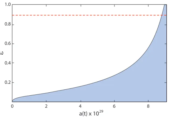
following Eq. 2.3 above), is shown in figure2. Indeed,2> bfor8.5×10−29.a.aend= 8.9×

10−29, but is far too small elsewhere forrpreCMBto exceed2rrec.

0 2 4 6 8

a(t) x 10

29

1.0

0.8

0.6

0.4

0.2

e

Figure 2.The small parameteras a function of the expansion factora(t)for the ‘small-field’ inflaton potential in Equation (2.16). The (red) dashed line marks the value required for the model to comply with thePlanckmeasurement

ofkmin.

An alernative characterization of such an evolution may be written in terms of the number of e-folds (Eq. 2.11) required during inflation in order to overcome the horizon problem, compared

to the actual number permitted by thekmin constraint in Equation (1.4). We have numerically

calculatedV (see Eq. 2.19 below) andN, subject to this constraint, for the following three

slow-roll potentials:

VQ(φ) = 1

2mφ

2

(Quadratic)

VH(φ) = V0[1−(

φ µ)

2

]2 (Higgs−like)

VN(φ) = V0[cos(

φ

f) + 1] (Natural). (2.17)

For specificity, we have continued to use the Planck optimized parameters. The principal

difference between our calculation and those carried out in previous work is the inclusion of Equation (1.4) as an initial condition. In addition, to this constraint, the other inputs informing

the calculation include: (1) the observed value of the scalar spectral index,ns= 0.96, which was

measured at the pivot pointkpivot≡0.05Mpc−1[3]; (2) an endpoint of inflation atV = 1(see

Eq. 2.19 below); and (3) a smooth transition from this inflated expansion to one driven by a radiation-dominated equation-of-state, as shown in Equation (2.8).

At the early stage of inflation, these potentials may be used to define an alternative set of ‘small

parameters’ηV andV [9], such that

(7)

7

rspa.ro

y

alsocietypub

lishing.org

Proc

R

Soc

A

0000000

..

0 15 30 45 60 1.0

0.8

0.6

0.4

0.2

e

Number e-folds

V

Quadratic

Higgs-like

Natural

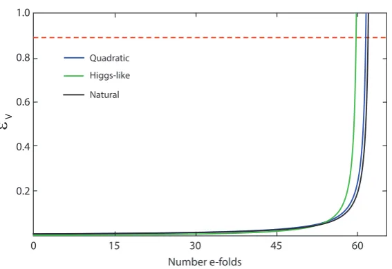
Figure 3.The small parameterVas a function of the number of e-folds (Eq. 2.11) for three illustrative slow-roll potentials

given in Equation (2.17). The (red) dashed line marks the value required for the model to comply with the Planck

measurement ofkmin.

where

V =

m2Pl

16π

V0 V

2

ηV =

m2_Pl

8π V00

V . (2.19)

The approximation breaks down whenV is large, which is conventionally taken to indicate the

end of the inflated expansion. The key results of our simulations are as follows:

•Quadratic:rpreCMB= 5,547Mpc, which is still a factor∼5too small compared to2rdec=

27,608Mpc. This potential would have expanded the Universe by 62 e-folds (see fig.3),

but 64 e-folds would have been required to fix the horizon problem. The difference of 2

e-folds accounts for the factor 5 difference betweenrpreCMBand2rdec.

•Higgs-like:rpreCMB= 3,339Mpc, which is a factor∼8too small. In this case, the Universe

would have expanded by 60 e-folds (fig.3), but a little over 62 e-folds would have been

required to mitigate the horizon problem.

•Natural:rpreCMB= 3,650Mpc, which is also a factor∼8too small. The Universe would have expanded by 63 e-folds, but a little over 65 e-folds would have been required to completely mitigate the horizon problem.

For direct comparison, the small parameterV is shown as a function ofNfor each of these

three inflaton potentials in figure3. As discussed earlier, inflation would have ended whenV →

1. As was the case in figure2, the horizontal red (dashed) line indicates the approximate value

V requires to comply with thePlanckmeasurement ofkmin, and we see that, whileV does cross

this mark in each case, it is not sustained at this high level long enough for the Universe to have expanded sufficiently to remove the horizon problem.

3. Slow-roll Inflation Preceeded by a KD or RD Fast-roll Phase

(8)

8

rspa.ro

y

alsocietypub

lishing.org

Proc

R

Soc

A

0000000

..

standard slow-roll expansion. A closely related problem to the missing correlations at large angles is the observed lack of power on the largest scales. Several authors have previously attempted to mitigate this problem by introducing additional features to inflation, such as the

aforementioned KD and RD phases. For example, ref. [11] showed that an early fast-roll inflation

can lead to a depression of the cosmic microwave background quadrupole moment, with a

characteristic scale k1∼(3,759 Mpc)−1 of the implied attractive potential. This is consistent

with our previously measured minimum cutoffkmin= (3,442 Mpc)−1. These authors did not,

however, simultaneously calculate the comoving distances rpreCMB and rdec to ensure that

rpreCMB≥2rdec. Subsequent work by these authors [12] to include both a decelerated fast-roll and an inflationary fast-roll phase similarly did not address the horizon problem in terms of the required comoving distances. In addition, this work appears to rely on the Bunch-Davies initial conditions, which may be problematic in the context of trans-Planckian physics.

This general approach was followed by other authors [13], who found that a fast-rolling

KD initial phase improves the primordial power spectral fit to the data, but they similarly

did not consider the impact of this treatment on rpreCMB versusrdec. Likewise, the Planck

Collaboration [14] considered the impact of a cutoff on the spectrum, though not the

angular-correlation function. Their treatment apparently also lacks a discussion of the possible impact of

such a cutoff onrpreCMBandrdec.

The work of ref. [15] was published after our measurement ofkmin[7], and they too considered

the impact of a sharp cutoff to the fluctuation spectrum. They concluded that the standard power-law is preferred by the data, but made no mention of the horizon problem and the lack of

correlations at large angles, however, and the impact of this approach onrpreCMBversusrdec.

An early phase of KD inflation was also introduced in ref. [16], though restricted to only

polynomial and exponential potentials. These authors confirmed that such a transition exhibits a generic damping of power on large scales, but did not explicitly consider its impact on the

angular correlation function andrpreCMBversusrdec.

The work that comes closest in spirit to our analysis in this paper is that reported in ref. [17].

These authors, however, considered specifically theλφ4potential and imposed the condition of

“just-enough" inflation. They found that the slow-roll conditions are violated at the largest scales, and that this approach cannot explain the lack of power at the largest angles. In subsequent

work [18], this treatment was expanded to include quadratic and hybrid-type potentials, but still

without a consideration of their impact on the angular correlation function.

Finally, ref. [19] analyzed how much inflation one should expect for a given energy scale of

order1016GeV. But this work lacks direct relevance to our proposed coupling ofkminmeasured

from the angular correlation function to the number of e-folds itself, and its bearing onrpreCMB

versusrdec.

Quite clearly, many authors have by now noted the glaring inconsistency associated with low power in the CMB fluctuations on large scales, which is closely related to their lack of correlation at large angles. Our work amplifies this general view by providing a much stronger

argument for a cutoffkminin the primoridal fluctuation spectrum, and its direct impact also on

the horizon problem itself. To complete this discussion, we shall now consider whether a KD or RD modification to the basic slow-roll inflationary picture can help mitigate the inconsistency

between rpreCMB andrdec when a cutoffkmin is invoked to suppress the correlation at large

angles.

We shall first follow a simplified approach in which we gauge the impact of a KD or RD

modification to the horizon problem based solely on the previously measured hard cutoffkmin. It

is well known, however, that the angular powerC`of each multipole`, from which the angular

correlation function C(θ) is calculated, depends on the entire fluctuation spectrumP(k) [7].

Thus, any modification to the power spectrum produced during the KD or RD phase alters

C(θ) from that expected under pure slow-roll conditions. Following our initial discussion of

the impact of KD or RD on the horizon problem using the previously measuredkmin, we shall

(9)

9

rspa.ro

y

alsocietypub

lishing.org

Proc

R

Soc

A

0000000

..

correlation function is re-optimized for a representative inflaton potential that contains a KD

phase transitioning into slow-roll at kstart. We shall find that kstart, signalling the start of

inflated expansion, can differ fractionally fromkminwhenC(θ)is fit to thePlanckdata, though

insufficiently to qualitatively alter any of the results.

We begin with a radiation-dominated Universe from the Big Bang to the onset of inflation, during which

H=Qa−2, (3.1)

whereQis a constant. Solving for the scale factor, one therefore has

a2= 2Qt , (3.2)

so that

dt=a da

Q . (3.3)

The comoving distance traveled by a photon during this period is therefore

rRD=c Ztstart

0

dt a =

castart

Q . (3.4)

Thus, combining this with Equation (3.1), we have

rRD=

c Hstartastart

. (3.5)

The addition of an RD period preceeding slow-roll inflation can therefore double the comoving distance travelled by a photon prior to the end of the inflation. Even this, however, is still far too small to solve the horizon problem, which requires the comoving distance to be at least 10 times bigger.

The addition of a KD fast-roll expansion may hold more promise. For such a scalar

field-dominated Universe, we have [9]:

H(φ)2= 8π 3m2_Pl

1 2 ˙

φ2+V(φ)

, (3.6)

and

¨

φ+ 3Hφ˙+V0= 0. (3.7)

From these two expressions, we derive

˙

H=− 4π

m2 Pl

˙

φ2, (3.8)

and

˙

φ=−m

2 Pl

4π H

0

. (3.9)

For a KD scalar-field potential, Equation (3.6) reduces to

H(φ)2≈ 8π

6m2_Pl

˙

φ2 (3.10)

and, solving forH, we find that

H(φ) =Hstarte 2√3π

m_Pl(φ−φstart)

, (3.11)

for which

H0=2

√

3π mPl

Hstarte 2√3π

m_Pl(φ−φstart)

. (3.12)

With Equation (3.9), we therefore find that

dt dφ=−

r

π

3 2

mPlHstart

e

2√3π

(10)

10

rspa.ro

y

alsocietypub

lishing.org

Proc

R

Soc

A

0000000

..

so that

t−ti= 1 3Hstart

e

2√3π

m_Pl(φstart−φ)

, (3.14)

wheretiis the time at which the KD expansion begins. Thus, with

˜

t≡t−ti, (3.15)

we also have

˜

t= 1

3H , (3.16)

during this phase prior to the onset of slow-roll inflation.

We may now solve for the scale factora(t), finding that

a=Mt˜1/3, (3.17)

so that

dt=dt˜=3a 2

M3da , (3.18)

whereMis another constant. Therefore, the comoving distance travelled by a photon during this

period is

rKD=c Z˜tstart

˜ ti

dt˜

a =

3c

2M3(a

2

start−a2i). (3.19)

As long as the KD period begins right after the Big Bang, we may therefore approximate this expression as

rKD≈ 3c

2M3a

2

start, (3.20)

and therefore we find, with the use of Equations (3.11) and (3.12), that

rKD≈

c

2astartHstart

. (3.21)

Clearly, even combining this comoving distance with that from the slow-roll inflationary period,

we find thatrpreCMBis still far too small to solve the horizon problem.

Finally, we consider all three phases together, beginning with an RD period, followed by a KD Universe and a subsequent slow-roll expansion. It is not difficult to show that

rRD+KD= 3c

2M3

a2start−a2?

+ca?

Q , (3.22)

wherea?is the scale factor at the RD to KD transition. Thus

rRD+KD=

1 + a

2 ?

a2_start

c

2astartHstart

< c astartHstart

. (3.23)

In the last step, we examine the possibility that a more careful calculation of the angular

correlation function C(θ) with a modified P(k) from the KD phase may yield an optimized

wavenumberkstart(signalling the start of inflation) differing from the hard cutoffkminwe have

been using in this analysis. It is not difficult to show from Equations (3.10-3.12) that the fluctuation

spectrum produced during KD isP(k)∼k3. To estimate the change one should expect to see with

this more detailed approach, we therefore now proceed to re-optimizeC(θ)with

P(k) =

(

As(k/k0)ns−1 ifk≥kstart

As(kstart/k0)ns−4(k/k0)3 ifk < kstart,

(3.24)

(11)

11

rspa.ro

y

alsocietypub

lishing.org

Proc

R

Soc

A

0000000

..

600

500

400

300

200

100

0

-100

-200

C

(

q

)

q

0 20 40 60 80 100 120 140 160 180

u = 4.34

u = 5.90

min

start

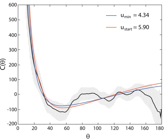
Figure 4.The best-fit angular correlation functions for P(k)with a hard cutoffkmin (blue) and forP(k)given in Equation (3.24) (red), with an optimized valuekstart= 4.12×10−4Mpc−1. These theoretical curves are compared to the angular correlation function measured withPlanck(dark solid curve) [14], and associated1σerrors (grey). (Adapted from ref. [7])

We follow the procedure outlined in ref. [7], and infer that the angular power of multipole`

relevant to the Sachs-Wolfe domain of fluctuations may be approximated as

C`=B Zustart

0

u ustart

3

j`2(u)

u du+B

Z∞

ustart

j2`(u)

u du , (3.25)

whereBis a normalization constant encompassingAsand several other factors; the variableu

is defined by the expressionu≡krdec, in terms of the comoving distancerdecto the decoupling

surface; andj`is the spherical Bessel function of order`. The angular correlation function itself is

then given by the expression

C(θ) =X `

(2`+ 1)

4π C`P`(cosθ), (3.26)

whereP`(cosθ)are the Legendre polynomials [20].

Using Equation (3.26) to refit the angular correlation function measured byPlanck[7,14], we

find that the optimized fit corresponds to the valueustart= 5.9. Thus, according to the definition

ofu, we find that

kstart= 4.12×10−4Mpc−1. (3.27)

In figure4, we show a comparison of the optimized angular correlation functions forP(k)with

a hard cutoffkmin(blue) andP(k)given in Equation (3.24) (red) with thiskstart. The curves are

almost indistinguishable, though the blue one is a slightly better fit to thePlanckdata at both small

(θ.45◦) and large (θ&120◦) angles [7]. This difference, however, is too small for us to decide

which of these fluctuation distributions is preferred by thePlanck data. Instead, the principal

outcome of this comparison is the change in wavenumber signalling the initiation of inflated

expansion: fromkminin Equation (1.2) for the hard cutoff, tokstartin Equation (3.27) for the KD

(12)

12

rspa.ro

y

alsocietypub

lishing.org

Proc

R

Soc

A

0000000

..

Thus, replacingkminin Equation (1.3) withkstart, and using Equations (2.6) and (3.23), we find

thatrpreCMB<4,848Mpc, which is still much smaller than the value (i.e.,27,608Mpc) required

to solve the horizon problem. In effect, the more detailed treatment ofP(k)has increasedrpreCMB

by about50%, but nowhere near the factor∼9required for this purpose.

No matter when the transition from RD to KD would have occurred, we find that no such modification to the basic slow-roll scenario can render inflation consistent with the measured

kmincutoff in the primordial fluctuation spectrum. The key point here is that, while introducing

a cutoff to the fluctuation distribution can account for the observed CMB anisotropies, it cannot simultaneously solve the horizon problem.

4. Conclusion

The most recentPlanckdata have affirmed the absence of large-angle correlations in the CMB

anisotropies, seen previously with several instruments over several decades. A prevailing view is that this feature may simply be due to ‘cosmic variance,’ based on the reasonable argument that we have only one Universe to observe, and that a variation away from its most probable configuration should not be unexpected. Certainly none of the work reported in this paper can completely eliminate that possibility. Nevertheless, seeking to find alternative explanations, as we have attempted to do here, is motivated by the presumed low probability of cosmic variance

being the sole answer. The analysis reported in ref. [7] shows that a more probable explanation

for the lack of large-angle correlations in the CMB is the presence of a hard cutoff kmin in

theP(k)spectrum. If true, this cutoff has profound consequences on the viability of slow-roll

inflationary models becausekmin points to a well-defined time at which inflation could have

started. Quantifying this impact on the possible form of the inflaton potential has been the main goal of this paper.

The constraint implied bykminallows inflation to simultaneously solve the horizon problem

and produce a near power-law fluctuation spectrum only if ≈1 throughout the inflationary

expansion. But such a scenario then predicts an extremely red spectral index completely at odds

with the measured value. Here, we have examined in detail the consequences ofkminon four

well-studied slow-roll inflationary models proposed thus far, showing that, if our interpretation

ofkminis correct, thePlanckCMB data rule out such slow-roll potentials at a very high level of

confidence.

Acknowledgments

FM is grateful to Amherst College for its support through a John Woodruff Simpson Lectureship.

Ethics Statement.This research poses no ethical considerations.

Data Accessibility Statement.All data used in this paper were previously published.

Competing Interests Statement.We have no competing interests.

Authors’ contributions.The authors together conceived the project, carried out the calculations, and wrote the paper. All authors gave final approval for publication.

Funding.None.

References

1. Wright E L Bennett C L Gorski K Hinshaw G and Smoot G F.1996. Angular Power Spectrum of

(13)

13

rspa.ro

y

alsocietypub

lishing.org

Proc

R

Soc

A

0000000

..

2. Bennett C L et al. 2003. First-Year Wilkinson Microwave Anisotropy Probe (WMAP)

Observations: Foreground Emission.ApJS14897.

3. Planck Collaboration. 2018. Planck 2018 results. VI. Cosmological parameters.A&Ain press

(eprint arXiv:1807.06209).

4. Guth A H. 1981. Inflationary universe: A possible solution to the horizon and flatness problems. Phys. Rev. D23347.

5. Linde A. 1982. A new inflationary universe scenario: A possible solution of the horizon,

flatness, homogeneity, isotropy and primordial monopole problems.Phys. Lett. B108389.

6. Copi C J Huterer D Schwarz D J and Starkman G D. 2009. No large-angle correlations on the

non-Galactic microwave sky.MNRAS399295.

7. Melia F and López-Corredoira M. 2018. Evidence of a truncated spectrum in the angular

correlation function of the cosmic microwave background.A&A618A87.

8. Mukhanov V F Feldman H A and Brandenberger R H. 1992. Theory of cosmological

perturbations.Phys. Rep.215203.

9. Liddle A R. 1994. Formalizing the slow-roll approximation in inflation.Phys. Rev. D49739.

10. Cook J L and Krauss L M. 2016. Large slow roll parameters in single field inflation.JCAP2016

028.

11. Destri C de Vega H J and Sanchez N G. 2008. CMB quadrupole depression produced by

early fast-roll inflation: Monte Carlo Markov chains analysis of WMAP and SDSS data.PRD78

023013.

12. Destri C de Vega H J and Sanchez N G. 2010. Preinflationary and inflationary fast-roll eras

and their signatures in the low CMB multipoles.PRD81063520.

13. Scacco A and Albrecht A. 2015. Transients in finite inflation.PRD92083506.

14. Planck Collaboration. 2016. Planck 2015 results. XIII. Cosmological parameters.A&A594A20.

15. Santos da Costa S Benetti M and Alcaniz J. 2018. A Bayesian analysis of inflationary primordial

spectrum models using Planck data.JCAP2018004.

16. Handley W J Brechet S D Lasenby A N and Hobson M P. 2014. Kinetic initial conditions for

inflation.PRD89063505.

17. Ramirez E and Schwarz D J. 2012. Predictions of just-enough inflation.PRD85103516.

18. Ramirez E. 2012. Low power on large scales in just-enough inflation models.PRD85103517.

19. Remmen G N and Carroll S M. 2014. How many e-folds should we expect from high-scale

inflation?PRD90063517.

20. Bond J R and Efstathiou G. 1984. Cosmic background radiation anisotropies in universes