Article
An Alternative for Indicators Which Characterize the
Structure of Economic Systems
Irina-Maria Dragan *,† and Alexandru Isaic-Maniu †
Department of Statistics and Econometrics, The Bucharest University of Economic Studies,
Bucharest 15-17 Dorobanti Avenue, District 1, Bucharest 010552, Romania; [email protected] * Correspondence: [email protected]; Tel.: +40-723-408-598
† These authors contributed equally to this work
Abstract: Studies on the structure of economic systems are, most frequently, carried out by the methods of informational statistics. These methods, often accompanied by a wide range of indicators (Shannon entropy, Balassa coefficient, Herfindahl specialty index, Gini coefficient, Theil index etc.) around which a wide literature has been created over time, have a major disadvantage. Such weakness is related to the imposition of the system condition, therefore the need to know all the components of the system (as absolute values or as weights). This restriction is difficult to accomplish in some situations, and in others, this knowledge may be irrelevant, especially when there is an interest in structural changes only in some of the components of the economic system (either we refer to the typology of economic activities - NACE or of territorial units – NUTS). This article presents a procedure for characterizing the structure of a system and for comparing its evolution over time, in the case of incomplete information, thus eliminating the restriction existent in the classical methods. The proposed methodological alternative uses a parametric distribution, with subunit values for the variable. The application refers to Gross Domestic Product values for five of the 28 European Union countries, with annual values of over 1,000 billion Euros (Germany, Spain, France, Italy and United Kingdom) for the years 2003 and 2015. A form of the Wald sequential test is applied to measure changes in the structure of this group of countries, between the years compared. The results of this application validate the proposed method.
Keywords: subunit distribution; structural analysis; statistical hypothesis; parameter estimation; sequential test
1. Introduction
A characteristic of our times, alongside globalization, is represented by knowledge transfer among different areas, resulting in the emergence and strengthening of border domains. Among the most interesting such domains is econophysics. In our field of interest is the second law of thermodynamics and its further developments, generated by the dispute between Max Planck and C. Caratheodory [1,2], leading to crystallization of the entropy concept. The entropy concept was introduced by L. Boltzmann (1844-1906), and the formula = ∙ , representing the dependency of the entropy S and probability W, engraved on the gravestone [3], requires a macro-system with known state probabilities ( ), but with the restriction: ∑ = 1. Debates and emulation generated by Gibbs Paradox, which showed a deviation from the second law of thermodynamics, generated a different approach of entropy [4].
Considered the father of informational theory, Claude Shannon proposed a new version of entropy calculus [5-7]: ( = − ∑ ∙ log with ∑ = 1.
Over time, Shannon entropy has diversify the types and the field of applications, such as: relative entropy, entropy of a composed system, conditional entropy, entropy of a correlated system, Tsallis entropy, Sharma-Taneja-Mittal entropy, Kaniadakis entropy, Abe entropy [8-10,2]. In parallel with the development of entropy indicator, was constituted a new group of such indicators used in the
analysis of the economic systems structure. A category of methods are the econometric ones, for example the Cobb-Douglas production function [11]: = ∙ ∙ ∙ ( where: Qt - total production output (the real value of all goods produced in a year); L - labor input (the total number of person-hours worked in a year); K - capital input (the real value of all machinery, equipment, and buildings); A - total factor productivity; t – time; α and β are the output elasticity of capital and labor, respectively. Also, in this category of methods it is framed the Input-Output model proposed by W. Leontief [12-14].
Among other specific methods, used in the analysis of the macroeconomic systems structure, are some quite significant. The Herfindahl index of regional specialization [15,16] is useful in analyzing the geographical distribution of territorial-administrative indicators, or the specializations in economic sector. Krugman index [17], in economic literature so called K-spec. index, assume dividing a country in geographical regions, or macro neighborhood, in the border areas of the European Union. K-spec. index, for a region, characterized contrasts that exist between the structure of the workload in a region and the defined area economy. The converted Gini index [18,19] is a statistical measure used for the analyzing the concentration among values of a frequency distribution. The benefit of this index is that it also applies to qualitative series (for example, production distribution by activity sectors NACE, income distribution by administrative subdivisions etc.). This coefficient is calculated as the ratio between the average of absolute deviations and the arithmetic mean of the items. The Gini index may also be computed based on a chart, according to the surface area of concentration, being its double. Gini index calculated against the per capita income is used to define types of countries such as OECD countries, the countries of Latin America, the countries of Eastern Europe. Theil index [20-22] is a statistical indicator, inspired by the entropy measurement, calculated for an uncertain event, characterized by a probability vector defined as the difference between the maximum value of the event entropy’s and its entropy. The Theil index value is directly proportional to the concentration of the distribution values, if the distribution is equiprobable, so the concentration is minimum, value of this index is zero.
The length of the structural vector x [23] is defined by ‖ ‖ : → , ∈ eventually ‖ ‖ = ∑ , with the limits ‖ ‖ = ∑ , respectively: ‖ ‖ =
√ ∑ .
It is estimated that its concentration is directly proportional to the indicator value, but it is recommended to take into consideration the following two observations: the indicator size is strongly influenced by the number of groups into which is divided the population and by the amplitude of the distribution, respectively, that the indicator is available into the measuring unit of the characteristic. For this reason, it cannot be used in comparing the concentration of population units relative to different characteristics.
The Lorenz curve [24,25] is used to characterize the diversification or concentration of information in an economic system. Concentration curve was used in the economic analysis, for the first time by Atkinson, to measure income distribution and redistribution, becoming in time "the golden standard". It is formed distinctly for discrete and continuous data. For a quantitative characteristic X defined by ( , , , where is a value, or a crowd, or an interval of values for the characteristic X, also is absolute frequency. In order to analyze the concentration of values for variable X, starting from the distribution ( , , , are calculated two sets of relative frequencies. The processing phases of a distribution, designed for analysis of the concentration degree, are represented below, distribution versus transformed distribution: ( , , ⟹ ( , , or
, ( , .
For curve fitting, where data series known ( , , , with the values for each characteristic, direct cumulative, are going through the next steps:
• The geographic regions are increasing arranged in relation to the values of the ratio ⁄
• For each variable, the relative frequencies and cumulative relative frequencies are calculated
• It’s drawn the Lorenz curve, by joining the points ( , ( , , where ( =
The concentration area, between the first bisector and the concentration curve, is a much more effective measure than a simple graphical representation, in order to characterize revenue distribution.
2. Materials and Methods
2.1. Statistical distribution
The class of statistical distribution usually defined on the interval (0, ∞ or , ]; , > 0 with applications to economic studies is extremely wide [26,27]. Excepting Beta distribution defined on 0,1] other few distributions defined on the same interval have been applied to the analysis of sub-unit economic indicators. For the analysis of economic phenomena, characterized by sub-sub-unit values (as, for example, the weights) we propose the probability density
: ( ; =1
2 (ln , ∈ (0,1], > 1 (1)
The restriction > 1 is necessary in order to have lim
→ ( , = 0 and to ensure the existence of the modal value on the stated interval (0,1]. Thus, the equation ( , = 0, i.e.:
( ; =1
2 ( − 1 (ln + (2 ln
1
2 = 0 (2)
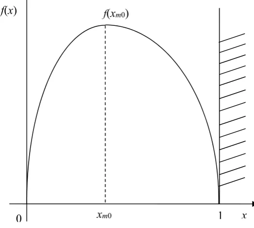
which is reduced to ( − 1 ln + 2 = 0 gives us the solution = 2/(1 − ]. If would be positive, but smaller than 1 – for instance = 1/2, we would get = > 1. So, the modal exists on (0,1] only if > 1 (for instance, for = 2, = 1/ , and (1/ = 16/ ).
The function graph is illustrated in figure 1.
Figure 1. Graph of f(x) function
The non-centered moment of n order is:
( =1
2 ∙ (ln = + (3)
providing the mean and dispersion under the forms:
( =
+ 1 , respectively ( = + 2 − + 1 (4)
(the fact that this expression is strictly positive can be easily verified).
f
(
x
)
0
f(
x
m0)
2.2. Estimating the distribution parameter
The estimation can be made by using the method of moments -Pearson [28], or by the maximum likelihood [29]. By applying the method of moments, we firstly estimate the theoretical non-centered n order moment. Consequently,
( =
2 ∙ (5)
According to calculations, in order to show that i=1, we get:
( =
+ (6)
Hence, the average and variance indicators follow immediately:
( =
+ 1 (7)
Respectively:
( =
+ 2 − + 1 (8)
Let , = 1, be a random sample of population {X}.
As 0 ≤ ≤ 1 for any i, we also have ̅ = ∑ ≤ 1. The estimation equation using the method of moments is therefore:
+ 1 = ̅ (9)
where
= ( ̅ /
1 − ( ̅ / (10)
The condition > 1 involving ̅ > = 0.125.
By using the maximum likelihood method, we immediately get: = ∑ ln whose
repartition is known.
Indeed, by making the transformation = , ≥ 0, our density becomes:
( ; , =
Γ( (11)
namely, a particular case of Gamma density [27,28,30]
( ; =
2 ∙ =Γ(3 (11’)
for k=3.
If parameter k is known, then:
1
= 1 (12)
3. Results
3.1. A particular case
We will analyze the particular case where = 2 (hence, the distribution is completely specified), in order to outline the difficulties met when calculating the distribution function for the general case. Indeed:
( ; ( ; =1
2 (ln (13)
and taking into account that [31] (p. 133):
(ln =
+ 1 (ln − + 1(ln + ⋯ + (−1 !
( + 1 + (14)
It follows for = 2, the expression = 1 obviously:
( ; 2 = 4 1
2 (ln −
1
2 ln + 1
4 (15)
Even for this simple case, the calculus of the theoretical median, for instance, leads to the transcendent equation ( ; 2 = 1/2, i.e. ( = (4(ln − 4 ln + 2 − 1 = 0 which really has a solution on the interval (0;1), as (0 = −1 and (0 = 1 and (0 ∙ (1 < 0. The solution is unique, as we can prove that the graphs of the curves ( = 4(ln − 4 ln + 2 and ( = 1/ are intersected in a single point on the interval (0,1).
The value of parameter = 2 is obtained, for instance, if ̅ ≈ 0.296 (from the estimation relation by means of the method of moments), a value higher than the “critical level 0.125”, in accordance [32] with equations (9) and (10).
Consequently, it is clear that the various problems related to the direct implication of the distribution function (quantiles assessment, natural tolerance, etc.) must be considered according to various particular values of , in order to finalize the computations. In the sequel, we proceed to developing the analysis using the sequential method.
3.2. Verifying certain statistical hypotheses Verifying a simple statistical hypothesis:
: = (16)
with the alternative:
: = ( < (16’)
has the significance of an hypothesis on the stability of the system structure at a given moment [28,32] by using the test of likelihood ratio with a single observation, we deduced the equation providing the decision constant according to and to the significance level of the test:
( ln − 1 + 1 = 2 ∙ (17)
In this equation, can be approximated either by a I-st degree polynomial (ln ≈ − 1 leading in the left side to a parabola
= ∙ − 2 ( + 1 + ( + 1 + 1 (18)
or by a II-nd degree polynomial ln ≈ − 1 − ( − 1 , leading in the left side to a IV-th degree curve (polynomial):
=
Again, the case where = 2 proves to be interesting, since we shall have to show that the polynomial = ( − 2 + 1 intersects only once the hyperbola = 2 / on the interval (0,1). Indeed, if we denote by ( = ( − 2 − + 1 we have lim
→ ( = −∞ and (1 = 2(1 − > 0 as 0 < < 1.
In the case we would like to use several sequels of observations, it is better to use the SPRT - Wald procedure (the developments in the area of theoretical and applied sequential analysis generated the editing of a profile journal since 1984: Sequential Analysis: Design Methods and Applications):
( =∏∏ ( ;( ; = ∙ (20)
which, by logarithms operation, leads to:
ln ( = 3 ln + ( − ln (21)
If and are the risks associated to the two hypotheses, A and B are the decision constants of the sequential test, ≈ (1 − / and ≈ /(1 − , then the experiment estimating area is given by the double inequality:
ln − 3 ln( / ]/( − < ln < ln − 3 ln( / ]/( − (22)
Here, , , … , , … is the sequential sample.
3.3. The sequential comparison
If we have two systems characterized by parameters and , then, from a practical point of view, it is interesting to compare the level of the respective parameters. This is reduced to verifying the compound hypothesis : ≤ versus the alternative : > .
Girshick [33] have proposed a SPRT test as follows: let X and Y be the two systems, or the same system in two periods (in our case), characterized by the densities ( ; and ( ; , respectively. We choose two values and ( < and let be the statistical hypothesis: the joint distribution of variables X and Y has the form ( ; ( ; , with alternative : the joint distribution is ( ; ( ; . In other words, verifying H versus H’ is reduced to: : = , =
: = , = .
By using the notations ( ; = ( ; ∙ ( ; and ( ; = ( ; ∙ ( ; , respectively, then the likelihood ratio associated to the observation pairs ( ; , ( ; , … , ( ; … is, in our case:
( ; = (23)
So, the uncertainty area is given by relations:
(ln /( − < ln < (ln /( − (24)
Girshick showed that reducing the verification of to that of can be made if there is a function ( ; with the following properties:
1. ( ; = 0 = 2. ( ; < 0 <
3. ( ; = − ( ;
Vaduva [34] proved that, for the distributions of type ( ; = ( ( + ( + ( , the Girshick’s function has the form ( ; = ± ( − ( ], where (+) or (-) appear when r is increasing/decreasing.
In case of our repartition, we can write:
( ; = ln 1
2 (ln = ( − 1 ln + ln(ln + (3 ln − ln 2 (25) hence ( ; = ( − ( = − 1 − ( − 1 = − , a function excellently meeting the conditions required by Girshicks’s method.
4. Application and Conclusions
The European Union's economy is emerging, year after year, growing stronger as a world leading economic player. In 2015, the total GDP of the 28 member states has exceeded 14,600 billion euro, accounting for around 20% of the world trade being, next to the US and China, the third world economic power.
We plan to look at whether, between the first five economies in the European Union (Germany, Spain, France, Italy, United Kingdom) with annual GDP values of more than 1,000 billion, there have been changes in the structure of the group. Table 1 shows the data for the years 2003 and 2015.
Table 1. GPD values for the analyzed group and total European Union
Country GDP – billion EUR Weight fi (%)
2003 2015 2003 2015
Germany 2,217 2,933 21.13 20.04
Spain 803 1,221 7.65 8.34
France 1,637 2,020 15.61 13.80
Italy
1,391 1,663 13.26 11.36United Kingdom 1,720 2,051 16.40 14.01
Total Group 7,768 9,888 74.05 67.55
Total UE 28 10,490 14,635 100.00 100.00
Source :http://ec.europa.eu/eurostat/statistics-explained/index.php/National_accounts_and_GDP/ro (accesed:15 .03.2017)
In 2015, the group of the most powerful economies in the European Union holds about 68% of GDP, compared with 2003, but also with weights changes.
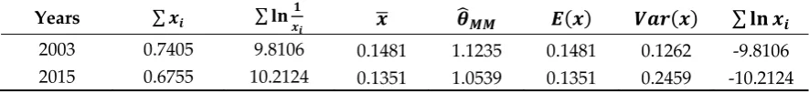
For example, the weight of Spain increased (+52.05% in 2015 compared to 2003), while for the rest of the group members the weights decreased, given the increase of GDP in absolute value (+27.29% for the group of developed country, respectively +39.51% across the European Union). The characterization of the structure using the methods of informational statistics (entropy, Gini coefficients, structure vectors, etc.) is not possible, because ∑ ≤ 1, but it is useful to use the method outlined above. The mean values determined by (3), the variants calculated by (4), the parameters computed by (10) and other intermediate elements necessary for testing the hypotheses (16), respectively (16'), and for determining the uncertainty intervals by (22), respectively (24), are presented in Table 2.
Table 2. Results of data processing
Years ∑ ∑ ( ( ∑
2003 0.7405 9.8106 0.1481 1.1235 0.1481 0.1262 -9.8106
Based on the information processed in Table 2, for the usual risks values of Type I and II, = 0.05 and = 0.10, with ln = ln 0.10/(1 − 0.05 and ln = ln (1 − 0.10 /0.05 , the decision report, the essence of the Wald test in the validation of the hypotheses (16) and (16'), through the interval established by (22) result: ∑ ln ∈ (−46.1298; 0.1344 , as in version (24), the size ∑ ln
is placed between the limits of uncertainty (−2.136 < 0.4020 < 2.74
The conclusion is that in the group of the five developed European Union countries, between 2003 and 2015, there were no major changes of the structure. This is a decision made at a type I risk of 5% or a type II risk of 10%.
Author Contributions: Authors contributed equally to this work.
Conflicts of Interest: The authors declare no conflict of interest.
References
1. Hendricks, V. F.; Jørgensen, K. F.; Lützen, J.; Pedersen, S. A., editors. Interactions: Mathematics, Physics and Philosophy, 1860-1930, Springer, Netherlands, 2006.
2. Pop, M. I. Some types of entropy and their applications. Ph. D. Thesis, Universitatea Transilvania, Brasov, 2012.
3. Koertge, N., editor in chief. New Dictionary of Scientific Biography. New York: Charles Scribner's Sons, 2007 4. Swendsen, H. R. Gibbs’ Paradox and the Definition of Entropy, Entropy 2008, 10(1), 15-18;
doi:10.3390/entropy-e10010015. Available online: http://www.mdpi.com/1099-4300/10/1/15 (accessed on 10 March 2017).
5. Höhn, A. P. Quantum Theory from Rules on Information Acquisition, Entropy 2017, 19(3), 98; Doi:10.3390/e 19030098.
6. Nanda, A. K., Paul, P. Some Properties of Past Entropy and their Applications, Metrika, 2006, Volume 64, Issue 1, pp 47–61. doi:10.1007/s00184-006-0030-6
7. Burgin, M. Information Theory: a Multifaceted Model of Information, Entropy 2003, 5(2), pp.146-160; Doi:10.3390/e5020146
8. Esteban M. D.; Morales D. A summary on entropy statistics, Kybernetika, 1995 Vol. 31, No. 4, pp.337-346. Available online: http://dml.cz/handle/10338.dmlcz/124679?show=full (accessed on 11 March 2017) 9. Scarfone, A. M., Wada, T. Thermodynamic equilibrium and its stability for microcanonical systems
described by the Sharma-Taneja-Mittal entropy, Physical ReviewE, 2005, APS Doi:10.1103/PhysRevE.72.026123, (accessed on 10 March 2017)
10. Keylock, C. J., Simpson diversity and the Shannon–Wiener index as special cases of a generalized entropy,
OIKOS, February 2005, Volume 109, Issue 1, pages 203–207, DOI:10.1111/j.0030-1299.2005.13735.x
11. Reiss, P., Wolak, F., Structural Econometric Modeling: Rationales and Examples from Industrial Organization, Chap. 64. In Handbook of Econometrics, 1st ed., Heckman, J. J., Leamer, E. E. (ed.), Elsevier, 2007; volume 6, pp. 147. DOI:10.1016/SI 573-4412(07)06064-3 2007.
12. Jackson, R. W., Integrating Input-Output and Life Cycle Assessment: Mathematical Foundation, Regional Research Institute Resource Document Series, 2013, Available online: http://rri.wvu.edu/resource-documents/
13. Gerking, D. S., Input-Output as a Simple Econometric Model. The Review of Economics and Statistics, 1976,
58(3), pp. 274-282, DOI: 10.2307/1924949, Available online: http://www.jstor.org/stable/1924949 (accessed on 11 March 2017).
14. Dobrescu, E., Restatement of the I-O Coefficient Stability Problem, Journal of Economic Structures, 2013, vol. 2, pp. 1-67. DOI:10.1186/2193-2409-2-2, Available online: https://link.springer.com/article/10.1186/2193-2409-2-2. (Accessed on 10 March 2017).
15. Aiginger, K., Davies, S. W. Industrial specialization and geographic concentration: two sides of the same coin? not for the European Union, Journal of Applied Economics, 2004, VII(2), pp.231-248, http://ageconsearch.umn.edu/bitstream/37627/2/aisinger.pdf (Accessed on 19 March 2017)
16. Midelfart-Knarvik, K.H., Overman, H. G., Redding, S. J., Venables, A. J. The Location of European Industry,
Economic Papers, Brussels, 2000, no. 142, pp. 67, Available online:
17. Krugman, P. Increasing Returns and Economic Geography, The Journal of Political Economy, 1991, vol.99 no.3,
pp. 483-499. Available online: https://www.princeton.edu/pr/pictures/g-k/krugman/krugman-increasing_returns_1991.pdf. (Accessed on 10 March 2017).
18. Sen, A., On Economic Inequality, Expanded Edition, Oxford University Press: New York, United States, 1997, Available online: https://www.scribd.com/document/285717503/79112317-Amartya-Sen-On-Economic-Inequality-Radcliffe-Lectures-pdf (Accessed on 10 March 2017)
19. Yitzhaki, S., Stochastic dominance, mean variance, and Gini’mean difference, American Economic Review,
1982, vol. 72, no. 1, pp.178-185 Available online:
https://www.researchgate.net/publication/4900733_Stochastic_Dominance_Mean_Variance_and_Gini%27 s_Mean_Difference. (Accessed on 11 March 2017).
20. Theil, H., The development of international inequality 1960-1985. Journal of Econometrics, 1989, 42,
pp.145-155. doi:10.1016/0304-4076(89)90082-1. Available online: http://www.sciencedirect.com/science/article/pii/0304407689900821, (Accessed on 9 March 2017).
21. Cowell, F. A., Measuring Inequality, Part of the series LSE Perspectives in Economic Analysis, Oxford University Press, 2009, Available online: http://darp.lse.ac.uk/Frankweb/MI3.htm. (Accessed on 11 March 2017).
22. Liston-Heyes, Cth.; Pilkington, A., Inventive concentration in the production of green technology: A comparative analysis of fuel cell patents, Sci. Public Policy, 2004, 31 (1), pp.15-25, https://doi.org/10.3152/147154304781780190, (Accessed on 13 March 2017).
23. Giraud-Héraud, E; Pichery M. C. editors. Wine Economics. Quantitative Studies and Empirical Applications,
2013, DOI :10.1057/9781137289520, Available online: https://link.springer.com/book/10.1057%2F9781137289520
24. Atkinson, A. B., On the Measurement of Inequality. Journal of Economic Theory, 1970, 2(3), p. 244-263. doi:10.1016/0022-0531(70)90039-6. Available online: http://www.sciencedirect.com/science/article/pii/0022-0531(70)90039-6. (Accessed on 9 March 2017)
25. Stiglitz, J. Walsh, C.. Economics, Fourh Edition, W.W. Norton & Co., New York, United States of America, pp. 869-885.
26. Burry, K. V. Statistical models in applied science, John Wiley & Sons, Ltd: New York, United States of America, 1975.
27. Balakrishnan, N., Nevzorov, V. B.. A primer on statistical distributions, John Wiley: New Jersey, United States of America, 2003, pp. 105-247.
28. Johnson, N. L., Kotz, S., Balakrishnan, N. Continuous univariate distribution, 2nd ed., John Wiley: New York, United States of America, 1995, pp. 337-396.
29. Everitt, B. S. Mixture Distributions—I. Encyclopedia of Statistical Sciences. 7., John Wiley & Sons, Inc.: United States of America, 2006.
30. Montgomery, D. C; Runger, G. C.; Hubele, N. F., Engineering statistics, 4th ed., John Wiley & Sons, Inc.: Hoboken, United States of America, 2010, pp. 138-141.
31. Wald, A. Sequential analysis, reprinted, Dover Publ, Inc.: New York, United States of America, 2004, p. 133. 32. Isaic-Maniu, A., Voda, Gh.V. A method for the analysis of sub-unitary parameters—an uniparametric
distribution, Economic Computation and Economic Cybernetics Studies and Research, 1987, 22 (3), pp.53-60. Available online: http://dl.acm.org/citation.cfm?id=48094&CFID=913660396&CFTOKEN=78318318. (Accessed on 11 March 2017).
33. Girshick, M. A. Contributions to the Theory of Sequential Analysis. I. Ann. Math. Statist., 1946, 17 no. 2, pp. 123--143. doi:10.1214/aoms/1177730976. Available online: http://projecteuclid.org/euclid.aoms/1177730976 (Accessed on 11 March 2017).