Article
A Comprehensive TCO Evaluation Method for
Electric Bus Systems Based on Discrete-Event
Simulation Including Bus Scheduling and Charging
Infrastructure Optimisation
Dominic Jefferies1,†* and Dietmar Göhlich1,†
1 Technische Universität Berlin, Department of Methods for Product Development and Mechatronics * Correspondence:[email protected]
† Current address: Technische Universität Berlin, Methoden der Produktentwicklung und Mechatronik, Straßedes17.Juni135,10623Berlin,Germany
Abstract: Bus operators around the world are facing the transformation of their fleets from fossil-fuelledtoelectricbuses.Twotechnologiesprevail: Depotchargingandopportunitycharging atterminalstops. Totalcostof ownership(TCO)isanimportantmetricforthedecisionbetween thetwotechnologies,however,mostTCOstudiesforelectricbussystemsrelyongeneralisedroute dataand simplifyingassumptions that maynot reflect localconditions. Inparticular, the need tore-schedulevehicleoperations tosatisfyelectricbuses’ rangeandchargingtimeconstraintsis commonlydisregarded.Wepresentasimulationtoolbasedondiscrete-eventsimulationtodetermine thevehicle,charginginfrastructure,energyandstaffdemandrequiredtoelectrifyreal-worldbus networks.TheseresultsarethenpassedtoaTCOmodel.Agreedyschedulingalgorithmisdeveloped toplanvehicleschedulessuitableforelectricbuses. Schedulingandsimulationarecoupledwitha geneticalgorithmtodeterminecost-optimisedcharginglocationsforopportunitycharging.Acase studyiscarriedoutinwhichweanalysetheelectrificationofametropolitanbusnetworkconsisting of39lineswith4748passengertripsperday.Theresultsgenerallyfavouropportunitychargingover depotchargingintermsofTCO,however,undersomecircumstances,thetechnologiesareonpar. Thisemphasisestheneedfordetailedanalysisofthelocalbusnetworkinordertomakeaninformed procurementdecision.
Keywords:Electricbus;busnetwork;simulation;scheduling;charginginfrastructure;depotcharging; opportunitycharging;optimisation;geneticalgorithm;TCO
1. Introduction
Municipal governments and public transport operators around the world have committed to transforming their fossil-fuelled bus fleets to zero-emission fleets, using either battery electric or fuel cell electric buses. The choice of technology has profound implications on the operational characteristics of the vehicles and the infrastructure required.
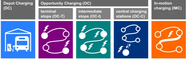
In recent years, significantly more battery electric buses were deployed than fuel cell buses, and the majority of bus operators in Europe appears to strategically favour this technology [1]. We therefore focus on battery electric buses in this work. However, even within the realm of battery electric buses, several charging strategies exist with vastly different operational characteristics (Figure1). We differentiate between depot charging (DC), opportunity charging at stationary charging points (OC) and in-motion charging (IMC). Opportunity charging can take place at terminal stops (OC-T), intermediate stops (OC-I) and at central charging stations (OC-C).
Opportunity Charging (OC) Depot Charging
(DC)
terminal stops (OC-T)
intermediate stops (OC-I)
central charging stations (OC-C)
In-motion charging (IMC)
Figure 1.Electric bus charging strategies
Opportunity charging at intermediate stops (OC-I) and at central charging stations (OC-C) is rarely encountered. In Germany, for example, only two electric bus projects (out of approximately 40 in total) used OC-I, one of which has been declared obsolete [2,3]. Our interviews with bus operators also suggest that OC-I is not desired due to the complex nature of planning infrastructure on public roads. OC-C has also seen only a few applications [1]. In-motion charging (IMC) is limited to cities that already have a trolleybus network, one exception being Berlin where building new trolley bus lines with in-motion charging is currently being discussed [4]. The majority of bus electrification projects focuses on depot charging (DC) and opportunity charging at terminal stops (OC-T)1.
For operators facing a decision between the two technologies, the total cost of ownership (TCO) is an important metric [5]. However, despite a wealth of publications dealing with the TCO analysis of electric bus systems, several aspects have received insufficient attention in the literature, as we will show in our literature review in Section3(after introducing a suitable structure for literature comparison in Section2). In particular, many works circumvent the problem of re-scheduling bus operations to satisfy the range and charging time constraints imposed by electric buses. This can lead to unrealistic results for the electric bus fleet size. The issue of increased staff demand is also commonly neglected. Most methods do not use real timetable and route data as an input, but generalised data. Delay data is not considered in any of the studies we evaluated, yet, as we will show, it has significant influence. We conclude from our literature evaluation that the existing methodologies are of limited applicability for bus operators planning the electrification of their fleet and seeking the most cost-effective option.
In Section4of this paper, we provide details on a simulation, planning and TCO assessment method first introduced in [6]. The method has since been further developed and currently includes
• an object-oriented, discrete-event simulation framework, enabling the energetic simulation of large bus fleets – including charging events en-route and in the depot – based on exact, non-idealised scheduling data,
• a scheduling algorithm to construct electric bus schedules adapted to range and/or charging time constraints and service delays,
• a genetic algorithm to enable cost-optimised placement of opportunity charging stations and • a TCO calculation module based on dynamic costing.
In Section5, we conduct a case study for a set of 39 real-world bus lines for which exact timetable, scheduling and delay data were available. By analysis of the existing (diesel bus) schedules, we will illustrate that a 1:1 exchange of diesel to electric vehicles often assumed in the literature is infeasible. We then apply the charging infrastructure optimisation and scheduling algorithms to construct fully electrified operational scenarios using depot and opportunity charging. The resulting vehicle schedules serve as input for a fleet and depot simulation that yields fleet size, fleet energy consumption, driver hours etc. These values are then fed into the TCO module to obtain total system cost for each scenario.
We close our paper with a discussion of our methodology and results (Section6) and a final conclusion and outlook (Section7). Detailed model equations are given in the Appendix.
2. General Workflow in Electric Bus System Planning and TCO Analysis
During recent years, an abundance of publications has emerged in the field of electric bus systems with very different scopes. Many publications focus on individual aspects of system design (for example, methods to obtain a feasible vehicle configuration or charging infrastructure layout for a given bus network) or system simulation (for example, vehicle energy consumption simulation). On the other hand, several publications deal with complete electric bus systems, mostly in order to compare different system configurations in terms of TCO. The latter studies vary considerably in the level of detail with which certain aspects are treated.
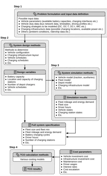
To facilitate a well-structured comparison of existing works, we propose a generalised representation of the electric bus system analysis workflow, illustrated in Figure 2. Based on comprehensive literature evaluation as well as our own developments, we identified four main steps:
1. Problem formulation and input data definition 2. System design methods
3. System simulation methods 4. TCO calculation methods
It should be pointed out that definitions in the literature may differ. For example, in our previous work [7], the entire process consisting of steps 1 to 4 is regarded assystem design. Generally, steps 2 to 4 are not semantically separated in the literature. They are also often not carried out sequentially, but simultaneously. This is especially the case in works utilising optimisation routines where some or all of the tasks are integrated into an objective function. For example, electric bus scheduling methods must incorporate some sort of vehicle model to determine energy consumption and vehicle range. In our generalised workflow, the scheduling algorithm is part of thesystem design methodsand the vehicle model contained therein is part of thesystem simulation methods. This separation of design and simulation aspects enables us to systematically compare existing methodological contributions, even if scope and context of the respective publications differ.
3. Literature Review
In the following subsections, existing works corresponding to each of the four steps introduced in Section2will be evaluated.
3.1. Problem Formulation and Input Data Definition
Many different problem formulations related to electric buses have been addressed in the literature (some examples were provided above). The selection of input data is highly dependent on the problem formulation. For instance, vehicle configuration – in particular, battery capacity – may be fixed and thus provided as an input parameter [6,8], or it may be part of the design problem [5,7,9]. The same applies to the location of charging infrastructure. An aspect of high practical relevance is the form of vehicle operation profile that is used as an input. Various types of operation profiles are observed:
• Driving profiles, i. e., a time series of velocity and elevation. These may be measured in real-world operation [10], taken from standard dynamometer driving cycles [7,11] or generated from microscopic traffic simulation [12].
Step 1
Vehicle parameters (available battery capacities, charging interfaces etc.) Vehicle duty data (bus network data, timetables, driving profiles etc.) Charging strategies to be modeled (DC, OC-T, OC-I, IMC etc.)
Charging infrastructure data (possible charging locations, available power etc.) Others (ambient conditions, ridership data etc.)
Possible input data:
● ● ● ● ●
Problem formulation and input data definition
Vehicle configuration Charging infrastructure layout Vehicle schedules
Charging schedules Etc.
Methods to determine:
● ● ● ● ● Step 2 Battery capacity
Location and capacity of charging stations
Number of depot chargers Vehicle schedules Etc. ● ● ● ● ● Design variables
Fleet mileage and energy demand Fleet size
Driver hours Vehicle states Charging station states Etc. ● ● ● ● ● ● Simulation results
Fleet size and fleet mix
Fleet mileage and energy demand Battery charging cycles
Driver hours
Number of charging stations Etc. ● ● ● ● ● ●
Full system specification
TCO results
Vehicle investment cost Infrastructure investment cost Maintenance cost Driver wages Interest rates Cost escalation Etc. ● ● ● ● ● ● ● Cost parameters System design methods
Vehicle model (traction, auxiliaries) Fleet model
Depot model
Charging infrastructure model Etc. ● ● ● ● ●
System simulation methods
Various costing models TCO calculation methods
Step 3
Step 4
arrival times; bus lines are commonly reduced to a single route variant2[5,8,9,13–15]. A slightly more detailed timetable representation is found in Keet al.[16] where absolute departure times and variable trip durations are considered, but resampled to 5-minute intervals.
Timetable data is often complemented with driving profiles to determine trip energy consumption [5,9,14,15].
• Exact bus line and timetable data.No simplifications are made to timetable data; any sequence of trips on any line and any route variant can be considered. This approach is common to all works specifically dealing with bus scheduling (see Section3.2), but seldom encountered in electric bus TCO studies, exceptions being Roggeet al.[17], Lindgren [18] and Jefferies and Göhlich [6]. • Transportation demand data.Some publications do not assume fixed timetables, but regard the
timetable as part of the design problem. They use demand data (e. g., passengers per hour) as an input [19,20].
3.2. System Design Methods
Depending on the problem description, considerably different methodologies are employed in this step. A common design task carried out in electric bus publications is to determine a feasible set of vehicle parameters, such as the battery capacity required for a given bus line [7,9,21] or a TCO-optimised battery capacity and/or charging power [22,23].
Also, various methods to determinecharging infrastructure locationshave been developed. They commonly use mixed-integer linear programming (MILP) and place charging infrastructure such that total system cost is minimised, e. g. [24,25]. Some approaches also simultaneously determine cost-optimised battery capacities [22,23]. Lindgren [18] uses an optimisation heuristic to determine charging infrastructure locations and then sets the vehicles’ battery capacities such that a certain lifetime is achieved. However, all aforementioned methodologies assume unchanged vehicle schedules. Their applicability is therefore limited to situations where charging at intermediate stops (OC-I), or, in the case of Lindgren [18] and Liu and Song [23], in-motion charging (IMC) is allowed. If charging is only desired at terminal stops (OC-T), a feasible solution may not be found depending on the dwell times available. Kovalyovet al.[20] formulate an optimisation problem to determine cost-optimised fleet mix, departure frequencies and charging infrastructure layout; however, no implementation is provided and it is thus unknown if real-world problem instances can be solved.
If it is not possible to operate existing vehicle schedules with electric buses – due to range or charging time limitations – the issue ofvehicle schedulingarises. We consider scheduling to be a central part of electric bus system design and a prerequisite for TCO analysis [6]. However, like the literature on charging infrastructure optimisation, publications dealing with electric bus TCO analysis often do not address the scheduling problem.
In TCO studies dealing with depot charging (DC), the scheduling problem is commonly circumvented by assuming that the daily distance covered by each vehicle does not exceed the electric buses’ range [11,26] or by setting a sufficiently high battery capacity, even beyond what is available on the market [13]. When treating opportunity charging (OC), the need for rescheduling is eliminated in several works by assuming charging at intermediate stops (OC-I) and deploying a sufficient amount of charging stations such that dwell times at the terminal stops can remain unchanged [5,9,13,18]3. These assumptions result in unchanged vehicle demand compared to the existing, conventional bus fleet. However, we have previously shown this not to reflect the reality of a metropolitan bus network [6] and will further elaborate on this in Section5.2.
2 It is common for bus lines to have full-length services operating “from end to end” as well as services operating on a shorter route inbetween, or to have several different branches. We term each of these aroute variant.
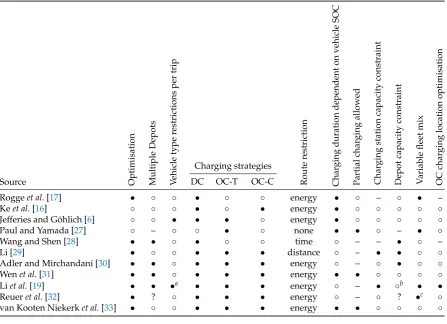
Table 1.Comparison of electric bus scheduling methods. Legend:•yes;◦no; – not applicable; ? unclear
Source Optimisation Multiple
Depots
V
ehicle
type
restrictions
per
trip
Charging strategies
Route
restriction
Char
ging
duration
dependent
on
vehicle
SOC
Partial
char
ging
allowed
Char
ging
station
capacity
constraint
Depot
capacity
constraint
V
ariable
fleet
mix
OC
char
ging
location
optimisation
DC OC-T OC-C
Roggeet al.[17] • ◦ ◦ • ◦ ◦ energy • ◦ – ◦ • –
Keet al.[16] ◦ ◦ ◦ • ◦ • energy • ◦ ◦ ◦ ◦ ◦
Jefferies and Göhlich [6] ◦ ◦ • • • ◦ energy • ◦ ◦ ◦ ◦ ◦
Paul and Yamada [27] ◦ – ◦ ◦ • ◦ none • • ◦ – • ◦
Wang and Shen [28] • • ◦ • ◦ ◦ time ◦ – – • ◦ –
Li [29] • ◦ ◦ • • • distance ◦ – • • ◦ ◦
Adler and Mirchandani [30] • • ◦ • • • energy ◦ – ◦ • ◦ ◦
Wenet al.[31] • • ◦ • • • energy • • ◦ ◦ ◦ ◦
Liet al.[19] • • •a • • • energy ◦ – • ◦b • •
Reueret al.[32] • ? ◦ • • • energy ◦ – ◦ ? •c ◦
van Kooten Niekerket al.[33] • ◦ ◦ • • • energy • • ◦ ◦ ◦ ◦
a This work differs from the others in that timetable creation is part of the problem formulation, so timetables are not given
explicitly. In constructing the timetable, however, different vehicle capacities are considered based on passenger demand.
b Overall fleet size constraint c Mix of diesel and electric buses
The aforementioned works do not provide a solution for depot charging if schedule lengths exceed vehicle range; neither do they allow opportunity charging exclusively at terminal stops (OC-T). The work by Pihlatieet al.[26] does deal with OC-T, but assumes sufficient dwell times are available to recharge at the termini. We have also shown this assumption not to hold true in real-world bus operation, especially if service delays are taken into account [6].
We are currently aware of only two contributions (other than our own) that determine electric bus system TCO utilising electric vehicle scheduling. Roggeet al.[17] developed a genetic algorithm to determine feasible, TCO-optimised schedules for depot charging, including a charging sequence at the depot minimising vehicle and charging infrastructure demand. This method yields a set of vehicle schedules that satisfies exact, real-world timetables and therefore enables a realistic determination of the resulting fleet size. However, it is applicable to depot charging (DC) only. In the TCO study by Keet al.[16], a scheduling algorithm for opportunity charging at central charging stations (OC-C) and depot charging (DC) is developed. Timetable data resampled to 5-minute intervals is used as an input. However, the algorithm does not consider the duration of deadhead trips – as a result, vehicles may be assigned trip sequences they cannot actually serve – and is subject to arbitrary restrictions, the rationale of which remains unexplained: Opportunity charging can take place only once an hour, and depot charging commences only after all vehicles have completed all trips.
an overview of these works as well as those already discussed above. They are compared with respect to the following criteria:
• Whether or not an optimal solution to the vehicle scheduling problem (VSP) is sought (column ”optimisation”).
• The ability to handlemultiple depots.
• The ability to specifyvehicle type restrictionsfor each trip. This is highly relevant to practical operation as different trips are often served by different vehicle types (e. g., small or large vehicles). • Thecharging strategiesconsidered (see Section1for their respective definitions).
• Whetherroute restrictionsare imposed in terms of energy (i. e., battery capacity), time or distance. • Whethercharging durationis evaluated based on the actual vehicle state of charge (SOC) or
assumed constant.
• Whetherpartial chargingis allowed or a full charge is assumed at each charging event.
• Whether charging stations and/or depots have a limited number of charging points (capacity constraints).
• Whether avariable fleet mixis determined, e. g. an optimal combination of short-range and long-range electric buses or an optimal combination of diesel and electric buses.
• Whether or not the approach determines the optimal location of OC charging stations (OC charging location optimisation).
Most works focus on finding an optimal solution to the VSP which, when considering battery capacity limitations, is NP-hard [29]. The central task in solving such problems is to develop feasible solution heuristics. Discussing these solution procedures is beyond the scope of this paper; it should be noted, however, that application is not always proven for large problem instances of several thousand trips. For example, the time-space-energy network approach by Liet al.[19] – the approach in Table1with the most general problem formulation – was not able solve an instance consisting of a comparatively small route network with four terminal stops, despite time being discretised to 30-minute intervals. The methods by Wen et al.[31] and van Kooten Niekerk et al.[33] were successfully applied to instances with around 500 trips, the method by Li [29] to around 900 trips. Adler and Mirchandani [30] demonstrated successful application for over 4000 trips and Reueret al.[32] for over 10000 trips. The approaches by Keet al.[16], Paul and Yamada [27] as well as our own [6] employ greedy algorithms and therefore do not yield optimal solutions, but are considerably less cumbersome to implement than optimisation methods and provide fast results even for very large problem instances. They are, however, applicable only to single-depot problems and are limited to DC and OC-T charging strategies.
As mentioned above, the ability to consider different vehicle types in the timetable is of great significance for real-world applications. Most works, however, do not enable this and would therefore require generating a separate problem instance for each vehicle type. This would provide feasible results only if capacity constraints and charging location optimisation are not part of the problem.
3.3. System Simulation Methods
In this section, existing methods for vehicle, fleet and depot simulation are compared.
3.3.1. Vehicle Modelling
The heating, ventilation and air-conditioning (HVAC) system is the most energy-consuming auxiliary device in an electric bus, its consumption potentially exceeding that of the drivetrain depending on weather conditions [7]. Despite this, most works related to electric bus system analysis and design do not model the HVAC system explicitly. Sebastianiet al.[15] do not consider the HVAC system at all. Hegazyet al.[35] perform vehicle simulations for various auxiliary powers, but they are not linked to a specific choice of HVAC system or specific weather conditions. Several authors use average overall vehicle consumption values, but do not state whether they include auxiliary consumption [8,13,16]. Lajunen [9] employs HVAC consumption data from Lajunen and Kalttonen [36], but it is unclear how the values were determined. Roggeet al.[17] employ a vehicle model from Sinhuberet al.[34] which uses measured values for auxiliary consumption (including the HVAC system). A detailed standalone HVAC system model was developed by the authors of this work [37,38], however its complexity impedes application within a fleet model. Kunith [5] uses this model to compute HVAC consumption for selected ambient temperatures prior to fleet simulation.
Explicit modeling of other auxiliaries in electric buses, such as air compressor, steering pump and battery heating/cooling, is – to the best of our knowledge – not encountered in the literature within the context of electric bus system analysis and design.
3.3.2. Fleet Modelling
We distinguish between two approaches to fleet simulation.Object-oriented or agent-based models using a discrete-event framework were popularised in autonomous taxi fleet and general logistics simulation [39–42], but are also applied to bus fleets [14,15,43,44]. All objects in the simulation – vehicles, charging stations, depots, etc. – are simulated simultaneously in a shared environment with a central simulation clock, each object having its own individual state. Events change the system state at discrete time steps and allow for communication between objects. The second approach issequential modelsin which vehicles do not share an environment and each vehicle’s state is evaluated separately [10,16,17]. Some models assume that all vehicles have a uniform operation profile [5,8,9,13], hence only one vehicle is evaluated and its energy consumption is multiplied by the fleet size.
3.3.3. Depot Modelling
Especially in the case of depot charging, the charging process at the bus depot can be a bottleneck with major influence on the e-bus fleet size (and therefore on TCO), as we will show in Section5.4. Several TCO studies, however, do not consider depot operations at all [8,9,13]. Some works approximate the additional vehicle demand arising from exchanging buses with depleted battery capacity and recharging them at the depot [5,45], but this specific approach is only applicable when using simplified timetable and route data (assuming constant travel duration and headway all day).
Rogge et al. [17] already consider the depot charging process at the scheduling stage (see Section3.2), hence its influence on fleet size is accounted for. However, as mentioned above, the methodology cannot handle opportunity charging.
A comprehensive electric bus depot model applicable to real-world bus schedules and any charging strategy is presented by Lauthet al.[46]. It is based on discrete-event simulation and considers all relevant processes at the depot, including cleaning, maintenance, parking, charging and dispatch.
3.4. TCO Calculation Methods
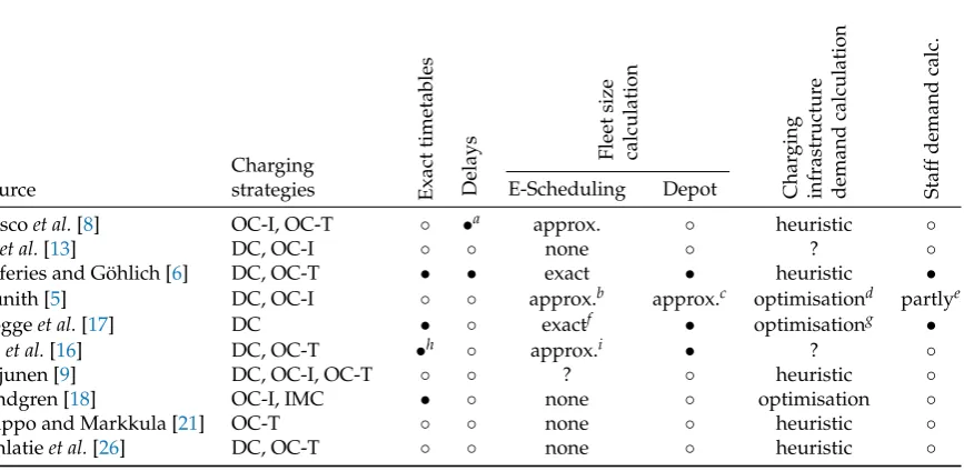
Table 2.Comparison of electric bus system TCO studies. Legend:•yes;◦no; – not applicable; ? unclear
Source
Charging
strategies Exact
timetables
Delays
Fleet
size
calculation
Char
ging
infrastr
uctur
e
demand
calculation
Staf
f
demand
calc.
E-Scheduling Depot
Fuscoet al.[8] OC-I, OC-T ◦ •a approx. ◦ heuristic ◦
Biet al.[13] DC, OC-I ◦ ◦ none ◦ ? ◦
Jefferies and Göhlich [6] DC, OC-T • • exact • heuristic •
Kunith [5] DC, OC-I ◦ ◦ approx.b approx.c optimisationd partlye
Roggeet al.[17] DC • ◦ exactf • optimisationg •
Keet al.[16] DC, OC-T •h ◦ approx.i • ? ◦
Lajunen [9] DC, OC-I, OC-T ◦ ◦ ? ◦ heuristic ◦
Lindgren [18] OC-I, IMC • ◦ none ◦ optimisation ◦
Vilppo and Markkula [21] OC-T ◦ ◦ none ◦ heuristic ◦
Pihlatieet al.[26] DC, OC-T ◦ ◦ none ◦ heuristic ◦
a Delays are considered implicitly by measurement of real trip durations. b For DC only
c For DC only
d Optimisation using MILP model e Only additional staff demand for DC f Full scheduling with genetic optimisation g Optimisation using MILP model
h Timetables are resampled to 5-minute intervals, but it may be assumed that the model can also operate with higher resolution
data.
i Simplified scheduling without deadheading
Aside from the type of costing model, the existing TCO studies also vary in the selection of cost components. While all studies include vehicle and infrastructure investment cost and energy cost, the following cost components are not always accounted for: Financing, driver wages, grid connection, vehicle and infrastructure maintenance, carbon emissions, salvage values.
3.5. Comparison of Electric Bus TCO Studies
Following our survey of individual methodological contributions to electric bus system design, simulation and TCO calculation, we will now analyse existing TCO studies that compare electric bus systems in their entirety. Table2lists some features of electric bus TCO studies:
• The charging strategies considered,
• whether exact timetable data is used as input,
• whether delays are considered during system design,
• whether bus scheduling is performed for fleet size calculation and in what manner, • whether charging at the depot is considered for fleet size calculation,
• how the location and/or number of required charging points is determined, • whether staff (i. e., driver) demand is part of the calculation.
For a bus operator facing a procurement decision between various electric bus system alternatives, it is desirable to determine the TCO of each electric bus systemfor the local operating conditions, i. e. the exact local routes and timetables, rather than for generalised or simplified cases that may not adequately reflect local conditions. We must conclude, however, that none of the methods discussed in this section can deliver this.
4. Electric Bus System Simulation and Planning Tool
To be able to perform a TCO comparison of electric bus systems for a real-world, metropolitan bus network, we developed eFLIPS4, a simulation and planning tool first presented in [6]. Development took place in multiple projects, not only in the context of electric buses, but also battery-electric trains and electric sanitation vehicles.
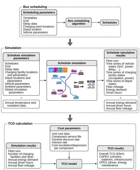
eFLIPS was implemented in Python [47] using strict object orientation. A discrete-event simulation framework was built using SimPy [48], a package providing a simulation clock, an event and process system, and capacity-constrained resources. Figure3gives an overview of the tool’s main features, the workflow involved in performing a TCO study as well as the inputs and outputs of each step. Each of the features will be explained in the following.
4.1. Bus Scheduling Algorithm
Our scheduling algorithm can plan schedules for depot charging (DC) and opportunity charging at terminal stops (OC-T). It follows a greedy approach similar to Paul and Yamada [27], but provides more flexibility: It can handle multiple vehicle types; it is possible to plan schedules for depot charging or refueling; in the case of opportunity charging, charging is not assumed ateveryterminus, but only at those stops defined as charging points. Like the algorithm by Paul and Yamada [27], it is limited to a single depot.
The main input to the algorithm is atimetable, i. e. a list of passenger trips sorted by departure time. A trip has the following attributes: Trip type (passenger or deadhead trip); vehicle type (e. g., standard or articulated bus); departure time; trip duration; delay; dwell time succeeding the trip5. Also, a list of charging locations and a set of vehicle parameters must be provided. The output is a list ofschedules, which, essentially, are also lists of trips, except they include deadhead trips and must only consist of trips of identical vehicle type.
The algorithm operates in two stages: First, schedules are built from successive trips without deadheading (other than the depot trips at the start and end of the schedule), i. e., the next trip must always begin at the destination of the previous. If the destination is a charging point, sufficient dwell time is provided to fully recharge the energy storage before the next trip commences. A global minimum dwell time can be specified. Optionally, delays can be added to the dwell time to ensure sufficient charging time and punctuality. After the addition of each trip, the vehicle SOC is evaluated. A schedule is terminated if one of the following is true: There are no more serviceable trips from the current destination (either no trips with a matching vehicle type are left at all, or those that are left exceed the maximum permitted dwell time); or, a critical state of charge is reached. In the latter case, trips are subsequently removed from the end of the schedule until the state of charge is valid. FigureA1in AppendixAshows a flowchart of this stage of the algorithm.
In the second stage, depicted as a flowchart in Figure A2 (Appendix A), it is attempted to concatenate the schedules created in stage I in order to maximise schedule length and to avoid unnecessary trips to the depot. The algorithm tries to join each schedule with the earliest reachable follow-up schedule through a deadhead trip until no more reachable schedules exist or a critical SOC
Bus scheduling
algorithm Schedules
Timetables Grid Delay data
Charging point locations Depot location
Vehicle parameters
Scheduling parameters
Bus scheduling
TCO model
Fleet size
Number of charging facilities and slots Annual energy demand Annual driver hours Annual fleet mileage
Simulation results
Unit cost data
Component service life General discount rate Interest rate
Cost escalation/degression per component
Cost parameters
Overall TCO (€/km) CAPEX (vehicles, batteries, infrastructure) OPEX (driver, energy, maintenance
TCO results
TCO calculation
Schedule simulation
Line 1 Line 2
Depot Simulation
Schedules Grid Delay data
Charging facility locations and parameters Depot locations and parameters Vehicle parameters Ambient parameters Global simulation parameters
Schedule simulation parameters
Annual temperature and insolation data
+
Fleet size
Time series of vehicle states (SoC, power, delay, ...)
Time series of charging facility states
(occupation, power) Time series of depot states
Fleet mileage Energy demand Driver hours
Schedule simulation results
Annual energy demand Annual driver hours Annual fleet mileage
+
Vehicle
Depot Dispatcher
Schedules Driver
Grid point Grid arc Charging point
drives along grid, computes energy consumption requests
charging facilities
drives vehicle according to schedule
assigns schedule and driver to vehicle
reads schedules
provides vehicle
requests vehicle
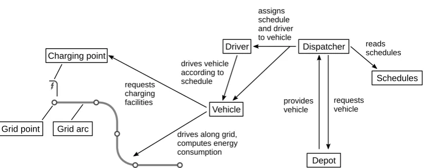
Figure 4.Simplified overview of the relationships between objects in the schedule simulation
is encountered. Similarly to stage I, the duration of the deadhead trip and the subsequent dwell time are capped to avoid excessive dwelling.
The distance of deadhead trips – i. e., depot trips and trips connecting different schedules – is determined through the openrouteservice car routing API [49]. A constant average speed is assumed to determine the duration of deadhead trips. For each of the two scheduling stages, it is possible to allow or disallow line changes.
4.2. Schedule Simulation
The schedule simulation forms the main component of eFLIPS. It enables simulation of any kind of predefined schedules using one of the four charging regimes introduced in Section1.
As pointed out above, the implementation follows an object-oriented approach. Thus, a schedule simulation replicates the physical objects encountered in the real world as depicted in Figure4:
• A list ofschedulesto be served is provided, as well as the geographicalgridcomprisinggrid points and connectingarcs. Typically, the schedules cover a single operational day, but any time window up to a week is possible.
• Theambient(omitted in Figure4) provides ambient temperature and insolation.
• Thecharging networkconsists ofcharging pointsfor stationary charging andcharging arcswhere vehicles can charge while in motion. Points and arcs each correspond to a point or arc in the grid, respectively. Charging facilities have a specificcharging interfacethrough which they can transfer energy to a vehicle. They are implemented as a SimPy resource with a defined capacity (i. e., the number of charging slots available). If a vehicle issues a charging request and all slots are occupied, it must queue for a free slot in order to charge.
• One or moredepotsexist where vehicles start and end their respective schedules.
• A centraldispatcherreads the list of schedules and, when a schedule is about to commence, requests a vehicle of the required type from the depot specified in the schedule. It also assigns a driverto the vehicle.
• Eachvehicleprovides various actions: Switching the ignition and air-conditioning on and off, driving along a specified leg of a schedule, driving along a specified velocity profile, modifying the payload (through boarding and alighting of passengers), etc. It has several sub-components, mainly the traction device, auxiliary devices and energy storage, as well as one or more charging interfaces. The vehicle model is explained in detail in Section4.2.2.
• Thedriverexecutes vehicle actions according to the schedule. It also keeps track of the time spent driving and idling.
Charge controller Energy storage m 1 Charging interfaces Loads Energy subsystem Vehicle Sub-components ● ● ● ●
primary energy subsystem
secondary energy subsystem (optional) charging logic driver Parameters ● ● ● ● ● vehicle ID vehicle type traction system parameters HVAC system parameters charging interfaces States ● ● ● ● ● ● ● location velocity
no. of passengers cabin temperature delay
heating/cooling load total power primary/ secondary ● ● ● ● SoC primary/ secondary ignition on/off HVAC on/off odometer, operation time, cumulated energy consumption, ... n 1 ... ... e.g.: Traction, HVAC, other auxiliaries e.g.: plug, pantograph
Energy flow port
● ● ● ● ● ● energy storage parameters kerb weight aux power (excluding HVAC) UA value insolation area cabin temperature
Figure 5.Vehicle and energy subsystem model
4.2.1. Discrete-Event Simulation Framework
The discrete-event system allows for communication between objects. For example, if a vehicle’s traction power changes, the traction device triggers a state change event. The vehicle’s charge controller listens for state change events and, upon receiving such an event, updates the energy flow to or from the energy storage. Similarly, charging facilities keep track of the total energy flow and the number of vehicles present. State change events also control when an object’s state is logged by the data logging system: The state of any object is only evaluated when it changes, saving computing time and memory.
4.2.2. Vehicle Model
A vehicle comprises a primary and, optionally, a secondaryenergy subsystem, each consisting of an energy storage, any number of connected devices(loads)– including traction, HVAC and other auxiliary devices – and any number of charging or refueling interfaces. Acharge controllerroutes the energy flow between loads, storage and interfaces. Upon each state change event, the energy storage integrates the net energy flow to determine the amount of energy charged or discharged. The structure of the vehicle and energy subsystem models is shown in Figure5. The primary subsystem always includes the traction motor; a secondary subsystem may be present, for example, if the heating system uses a different fuel than the traction motor, as is the case in electric buses with diesel-fueled heating. Two traction models are available for simulation (cf. Section 3.3.1): A constant specific consumption model that determines energy consumption on a per-arc basis, and a longitudinal dynamics model requiring a driving profile. The latter currently cannot be used for schedule simulation, however it is used to determine typical mean consumption values for standard driving cycles that can later be used in a schedule simulation.
Several HVAC component models were implemented using parameters from manufacturers’ data: Electric heat pump, electric air conditioning, electric resistance heater and diesel heater can be combined to several HVAC system configurations. Auxiliaries other than the HVAC system are modelled as one device with constant power.
queue for
charging slot manoeuvreto charging position
dock interface charge undock interface
wait for departure
P
manoeuvre to parking
position
P
Figure 6.Actions controlled by charging logic
Vehicles in service
Vehicles in depot
Vehicle demand: 4 vehicles
time
► New vehicle object generated
► Vehicle 1: Schedule 1
► Vehicle 4: Schedule 4 ► Vehicle 3: Schedule 3
► Vehicle 2: Schedule 2
Vehicle 1: Schedule 5
Vehicle 2: Schedule 6
Vehicle 1
Vehicle 2
Vehicle 3
Vehicle 4
Vehicle 1
Vehicle 2
State of charge (SOC)
Figure 7.Vehicle demand calculation
the charging logic are depicted in Figure6. Queuing and manoeuvring are generally only applicable to stationary charging points. Various queuing strategies can be defined: Vehicles can queue for a free charging slot or skip charging if all slots are occupied; also, vehicles can release the charging slot once they are fully charged, or remain at the charging point until departure. These features were implemented to be able to evaluate the impact of different driver break regulations on charging infrastructure demand. It is also possible to force vehicles to always wait until fully charged (even if this causes a delay), or to depart as punctually as possible (even if this leaves no time to charge).
Furthermore, several energy storage (battery, diesel tank) and charging interface models (stationary pantograph, trolleybus pantograph, CCS plug, diesel nozzle, train pantograph) were implemented. When connected to a charging interface, a constant charging power is assumed.
A full documentation of the model equations is given in AppendixC.
4.2.3. Depot Model
Vehicles start and end their schedules at a depot. Any number of depots can be defined in the simulation. Each depot keeps track of the number of vehicles currently in service and the number of vehicles present at the depot for charging and parking. All depots are empty at the start of the simulation. If a vehicle is requested for line service from a depot by the dispatcher, the first available vehicle currently parked at the depot is chosen; if no vehicle is available, a new vehicle is generated and added to the depot. Thus, the required fleet size can be determined by counting the number of vehicles generated in total by the end of the simulation, as illustrated schematically in Figure7.
t
tstart tend
(a) Investments
CAPEX
CCAPEX,c(t)
tbase
∆tdp,c ∆tdp,c
t
tstart tend
CFCAPEX,c(t)
tbase
(b) Cash flows (annualised)
t
tstart tend
CFCAPEX,NPV,c(t)
tbase
(c) Cash flows discounted to base year
OPEX
t
tstart tend
CFOPEX,c(t)
tbase
(d) Cash flows (e) Cash flows discounted to base year
t
tstart tend
CFOPEX,NPV,c(t)
tbase
∆tproject
Figure 8.TCO calculation method
power. After charging, vehicles are again blocked for a certain dead time before being able to return to service.
4.3. Year Simulation and TCO Calculation
To determine the fleet’s annual energy demand required for TCO calculation, it is important to consider the seasonal variation of HVAC system consumption. Thus, a batch simulation module was developed allowing simulation of any number of parameter sets. We use the batch simulation module to determine annual simulation results on the basis of a year’s temperature and insolation function. Both functions are discretised intonintervals such that a listTof temperature and insolation values and the respective number of days (i. e., the width of the interval) is produced:
T=(Ndays,1,T1, ˙qsol,1), . . . ,(Ndays,n,Tn, ˙qsol,n)
. (1)
For each quantityQobtained from a schedule simulation for one single day, the annual quantityQais obtained through
Qa= n
∑
i=1Ndays,iQ(Ti, ˙qsol,i), (2) whereQmay be the fleet energy consumptionEfleet, fleet mileageMfleetor driver hours∆tdriver.
Vehicle and infrastructure demand are not determined from the year simulation, but from a separate schedule simulation using a critical consumption case (usually a very cold winter day).
The overall system TCO is obtained by summing up all discounted cash flows. A full description of the calculation can be found in AppendixD.
4.4. Genetic Algorithm for Charging Infrastructure Optimisation
The functions of eFLIPS presented thus far – electric bus scheduling, schedule simulation, year simulation and TCO calculation – require the specification of charging infrastructure locations as an input parameter. In the case of depot charging, this is trivial. When dealing with opportunity charging, however, deciding upon the location of charging points can become a complex task: As any combination of charging points poses a separate scheduling problem, the effect of charging point positions on overall system cost is difficult if not impossible to predict by intuition. Also, real-world bus networks produce solution spaces of considerable magnitude, as our case study presented in Section5will illustrate. It therefore seems purposeful to develop an optimisation method to determine a cost-optimised set of charging locations for opportunity charging.
To enable this, the entire process shown in Figure3was wrapped into a single function that returns the TCO of an electric bus system, using timetable data and charging point locations as the main inputs. A binary genetic algorithm (GA) was implemented that uses this aggregated TCO function as a fitness function.
A list of possible locations for OC charging infrastructureL = (l1, . . . ,li, . . . ,lNloc)defines the lengthNlocof each chromosomec= (b1, . . . ,bi, . . . ,bNloc). The positioniof each allele maps to location liand the value of the allele indicates whether a charging station is present at this location (bi =1) or not (bi=0). A population sizeNpopis defined and an initial population is generated randomly. For each new generation, the bestNkeep =xselectNpopchromosomes are kept,xselectbeing the selection share, and the rest is discarded. Chromosome pairs (parents) are randomly selected to produce offspring through single-point crossover until the original population size is reached. The offspring is then mutated using the mutation rateµ. We defineµas the share of alleles that is randomly modified, i. e.,Nmut=d(Nchrom−1)Nlocµealleles at random positions are switched,Nchrombeing the number of chromosomes in the population subset that mutation is applied to.
The number of charging slots is set to an arbitrary, high value for all stations in the schedule simulation so that, effectively, no capacity constraints exist. This is because the scheduling algorithm currently does not support charging station capacity constraints.
To reduce computation time, a simplified TCO calculation method was adopted for the GA fitness function: Instead of performing a year simulation using a temperature distribution, annual energy consumption is obtained by simply multiplying energy consumption for the critical consumption case by 365. Also, a static costing model is used.
Further reduction in computation time is obtained by skipping the fitness evaluation of infeasible solutions: Solutions not including at least one charging location per bus line are penalised by being assigned a very low fitness (i. e. high cost) value. Their actual TCO is not evaluated. Also, the algorithm caches all chromosomes and their respective fitness values such that no chromosome is evaluated twice. Parallel processing support was realised using Python’smultiprocessingpackage.
5. Case Study: Electrification Scenarios for an Urban Bus Network
To illustrate the application of our methodology, we conducted a case study for a real-world bus network consisting of 39 lines, of which 28 operate at daytime, 2 provide 24-hour service and 9 are night lines. For these lines, the current diesel bus schedules – from which the timetables can be generated by discarding the empty trips – and delay data were made available by the bus operator.
5.1. Vehicle Specifications and Energy Consumption
Table 3.Parameters used for longitudinal dynamics simulations
Quantity Symbol Value Source
Rolling resistance coefficient fr 0.0075 [51]
Drag coefficient cw 0.66 [34]
Frontal projection area Afront 8.8 m2 [34] Rotational mass factor λ 1.1 [5]
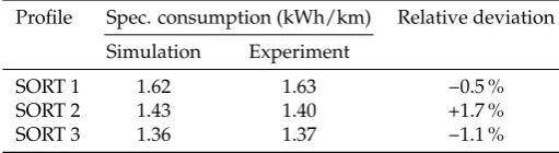
Table 4. Comparison of simulated and experimentally determined energy consumption for SORT cycles
Profile Spec. consumption (kWh/km) Relative deviation
Simulation Experiment
SORT 1 1.62 1.63 −0.5 %
SORT 2 1.43 1.40 +1.7 %
SORT 3 1.36 1.37 −1.1 %
cycles by longitudinal dynamics simulation. The specific consumption obtained in this manner is later used for the constant consumption model in the schedule simulation.
5.1.1. Parameterising the Longitudinal Dynamics Model
Detailed SORT [50] test data was available from a bus manufacturer for an 18 m articulated electric bus. The test yields specific vehicle consumption in kWh/km for a SORT 1, 2 and 3 cycle using a fixed payload. These experimentally determined consumption values were used to parameterise and validate the vehicle model presented in AppendixC.
The parameters fr,cw,Afrontandλused in Eqs. (A25) and (A26) were obtained from literature (Table 3). The HVAC system power PHVAC is zero because the HVAC system was switched off during the SORT test. This leaves the total drivetrain efficiencyηtotal in Eq. (A23) and the power of the remaining auxiliariesPaux,otherin Eq. (A2) unknown. They were determined by least-squares approximation such that
3
∑
i=1eSORT,i,sim−eSORT,i,exp 2
→min, (3)
wherei = 1 . . . 3 corresponds to the respective SORT profile,eSORT,i,simis the specific consumption obtained from longitudinal dynamics simulation andeSORT,i,expis the experimentally determined specific consumption. The least-squares approximation yieldedηtotal=0.86 andPaux,other=5.40 kW, both of which are plausible (e. g., by comparison with Sinhuberet al.[34]). Using these parameters, the SORT cycle energy consumption obtained through simulation was within 2% of the experimentally determined consumption, as Table4indicates. The parameters will thus be used henceforth.
5.1.2. Defining Vehicle Types for the Simulation
We defined five base types of electric buses: Three depot charging types with low (120 km), medium (200 km) and high (300 km) range, and two opportunity charging types with a range of 60 km and different charging powers (300 kW and 450 kW). For each base type, parameters for a standard 12 m bus and an articulated 18 m bus were defined, yielding 10 electric bus configurations in total.
permit solving for the battery capacity explicitly. The resulting battery weight was determined using energy density values taken from current manufacturer datasheets; for the high-range depot chargers, a 20% increase in energy density was assumed. Lithium-ion NMC batteries were assumed for the depot chargers and LTO batteries for the opportunity chargers. Vehicle base weights (without battery) were obtained as mean values from the literature. The full set of vehicle parameters used henceforth is listed in Table5.
5.2. Simulation of Existing Schedules With Electric Buses
To assess the operability of the existing diesel bus schedules with electric buses, we performed simulations of the 317 unchanged schedules that cover the 39 lines on a weekday. Five scenarios, each corresponding to one of the vehicle types in Table5, were simulated. Critical consumption parameters (SORT 2, 50% occupation, −10 °C outside, 17 °C inside) were assumed as outlined in the previous section.
For the opportunity charging scenarios, the location of charging stations6has to be defined. The charging optimisation algorithm introduced in Section4.4cannot be applied in this case because it enforces rescheduling of the vehicles. To avoid subjective decisions, a simple heuristic was chosen: A charging point was assumed ateveryterminus, even at termini that are only seldom visited. This yielded a total of 128 OC charging stations (more than 3 stations per line). It must be noted that this approach does not in any way reflect operational practice; it simply constitutes the upper boundary in terms of available energy supply and thus can be considered a theoretical best-case scenario for OC.
For the simulation of existing schedules, the question of interest is whether vehicles can sustain a valid state of charge during schedule operation. Depot operations are irrelevant at this stage. Thus, no depot simulation was carried out; a new, fully charged vehicle was generated for each schedule. If vehicles arrived at a terminus delayed, the dwell time (and, therefore, the charging time in the OC cases) was shortened to permit a punctual departure whenever possible.
Simulation was carried out for punctual and delayed operation. For the latter case, historical delay data was available from the bus operator; the delay assigned to each trip was obtained as the 90th percentile of all delays observed on similar trips within the same hour of the day7.
The simulation results are shown in Figure9. It is observed that delays exert only a minor influence in the depot charging scenarios; in the opportunity charging scenarios, however, the results change considerably when delays are taken into account. As expected, the higher the DC vehicles’ range and the higher the OC vehicles’ charging power, the more schedules can be served. There is, however, no scenario that permits electric bus operation with completely unchanged schedules. Also, it must be emphasized that the OC results for a more realistic charging infrastructure setup would be considerably worse. These results reinforce our point that the transition to electric buses in a metropolitan bus network requires a re-scheduling of vehicle operations [6].
5.3. Fully Electrified Scenarios: Scheduling and Charging Infrastructure Optimisation
We will now proceed to construct scenarios for fully electric bus operation. Six scenarios were generated: Five electric bus scenarios corresponding to the vehicle types in Table5and a diesel reference scenario for comparison. Diesel vehicles were modelled using a specific average consumption of 44.4 litres/100 km for standard buses and 59.4 litres/100 km for articulated buses (values from a bus operator’s fleet consumption evaluation over an entire year). HVAC system and other auxiliaries were not modelled for diesel buses, they were included in the average consumption.
For each of the scenarios, a new set of schedules has to be generated. In order to invoke the scheduling algorithm presented in Section4.1, we first have to define a timetable. This is achieved
DC (120 km)
punctual
93 (29%) 7 (2%) 217 (68%)
DC (200 km)
129 (41%)
6 (2%) 182 (57%)
DC (300 km)
245 (77%) 14 (4%)58 (18%)
OC (300 kW)
315 (99%) 2 (1%)
OC (450 kW)
315 (99%) 2 (1%)
delayed
93 (29%) 4 (1%) 220 (69%)
128 (40%)
6 (2%) 183 (58%)
244 (77%) 10 (3%)
63 (20%)
260 (82%) 57 (18%)
290 (91%) 27 (9%)
OK
critical
invalid
Figure 9. Results from the simulation of existing diesel bus schedules with electric buses. The pie charts indicate the number of schedules for which the following applies: Green – schedules can be served within the SOC limits of the battery and also leave an operational safety margin of 10 km; yellow – schedules can technically be operated, but violate the 10 km safety margin; red – schedules are inoperable because they violate the SOC limits of the battery.
by filtering the existing schedules for passenger trips on the specified lines. For the daytime lines, all trips during a weekday were chosen (this typically includes all trips between 4:00 AM and 1:00 AM of the following day). For the night lines, all trips departing on the evening of the same weekday and during the following night were considered. For the 24-hour lines, a time window must be chosen. We considered all trips departing between 03:00 AM and 02:59 AM on the following day, in accordance with the bus operator’s definition of an operational day. The resulting timetable consists of 4748 trips. All trips shall be served by a single depot.
For scheduling, the minimum dwell time was set to zero as some lines currently operate with zero dwell time at certain termini. Maximum dwell time and maximum deadheading time were set to 45 minutes. The average velocity used to compute the duration of deadhead trips was defined as 25 km/h. Line changes were only permitted during the second stage of scheduling (cf. Section4.1). A reserve range of 10 km was assumed for all vehicle types and the effective battery capacity available for scheduling was reduced accordingly.
Delays were taken into account in all scenarios during scheduling: The minimum dwell time at every terminus was increased by the delay upon arrival such that a punctual departure for the succeeding trip is always possible. Technically, it would also be conceivable to consider delays only in the case of OC, since only OC requires “guaranteed” dwell times for recharging even in the presence of delays. However, this would imply the OC systems can maintain a higher level of punctuality than the DC and diesel systems. To ensure a consistent quality of service for the passenger in all scenarios, it is thus appropriate to always consider delays.
(a)300 kW scenario
0 200 400 600 800
Generation 4.6
4.7 4.8 4.9
Cost (
/km)
0 20 40 Time (h)60 80 100 120
(b)450 kW scenario
0 200 400 600
Generation 4.6
4.7 4.8 4.9
Cost (
/km)
0 20 40 Time (h)60 80 100 120
Figure 10.Progress of charging infrastructure optimisation
Table 6.Scheduling statistics
Case Number of schedules Mean distance (km) Mean duration (h) Mean efficiency (%)
DC (120 km) 667 96.7 5.9 88.2
DC (200 km) 441 138.6 8.6 91.5
DC (300 km) 350 171.2 10.7 92.8
OC (300 kW) 340 176.1 12.3 93.3
OC (450 kW) 327 182.3 12.4 93.4
Diesel 302 195.8 12.3 93.7
Xeon E5-2640 machine with 64 GB RAM was used. Figure10shows the TCO of the best solution per generation over the course of the iteration8.
The genetic iteration yielded a set of 42 charging locations for the 300 kW scenario and 44 charging locations for the 450 kW scenario. These configurations were subsequently used for schedule generation and system simulation. Further discussion of the charging network optimisation results is found in Section6.
The results of the scheduling process are listed in Table 6. The scheduling efficiency was determined for each schedule as the ratio
ηschedule = tproductive ttotal
, (4)
wheretproductiveis the time spent during revenue service, i. e. on passenger trips excluding pauses, andttotalis the total operation time. Computing time for schedule generation was 333 seconds, or≈56 seconds per scenario, on an Intel Core i5-6200U using a single core.
As would be expected, in the case of DC, the lower the vehicle range, the more schedules were generated and the lower is the resulting schedule efficiency. This is because more depot trips are required for the same number of passenger trips. The OC schedules provide higher efficiency than the DC schedules, indicating that the unproductive time for recharging OC vehicles is lower than the unproductive time for additional depot trips in the DC case. Diesel schedules have the highest mean efficiency and distance.
5.4. Fully Electrified Scenarios: System Simulation
The schedules generated for each technology in the previous section serve as the main input for the system simulation. The goal of the system simulation is to obtain the number of vehicles and charging points required to operate the schedules under critical conditions (a cold winter day as outlined in Section5.2). Each individual vehicle is simulated; example SOC plots from a single-day simulation are given in Figure11.
Schedules were generated for five electric bus scenarios (scenarios 1–5) and a diesel reference scenario (scenario 8) as illustrated in the previous section. Two additional electric bus scenarios (scenarios 6 and 7) not requiring additional scheduling were simulated to observe the impact of reducing the charging power at the depot: The medium range DC scenario and the low power OC scenario are replicated with a depot charging power of 60 kW instead of 150 kW.
To correctly simulate depot operations, the schedules have to be repeated twice such that a period of three consecutive days is simulated as illustrated in Figure12: Only on the second day will there exist an equilibrium state that reflects actual weekday depot operation. This is because at the beginning of the simulation, the depot starts empty and it takes some time until all vehicle objects have been generated; at the end of the simulation, all schedules have ended andallvehicles are returned to the depot. In reality, this never happens because a certain number of vehicles is always in service at any time of day.
The number of required fast charging slots was obtained as the sum of the maximum occupation of each charging station; an example is provided in Figure13. The number ofavailableslots per station was set to a high value in the simulation so that, effectively, charging station capacity was unconstrained. Vehicles were configured to occupy their charging slot until departure9. The required number of depot charging slots was determined from the maximum depot occupation as illustrated in Figure12. One depot charging slot per vehicle was assumed.
The simulation results are presented in Table7. We observe the following:
• Generally, the electric bus scenarios require at least 20 more vehicles (+12%) compared to the 234 vehicles in the diesel reference scenario. The only exception is the long-range DC scenario (scenario 3) that requires only 3 more vehicles (+1.3%).
• Reducing the charging power at the depot from 150 kW to 60 kW incurs a significantly larger fleet in the case of depot charging (+14 vehicles or 4%). In the case of opportunity charging, the increase in fleet size is less pronounced (+2 vehicles or 0.8%).
• Increasing the DC vehicles’ range from 120 to 200 kmincreasesthe required fleet size substantially by 32 vehicles or 10%. This is because in the 200 km case, many vehicles run out of energy during the afternoon when vehicle demand is at its peak and, thus, many new vehicles have to be generated. In the 120 km case, however, most vehicles return to the depot for charging before the afternoon peak and can then cover the entire afternoon shift uninterrupted. This surprising result illustrates the limits of the greedy scheduling algorithm: The objective pursued by the algorithm to maximise schedule length does not necessarily lead to a minimum fleet size.
5.5. Fully Electrified Scenarios: TCO Comparison
For the final step of our analysis, the TCO comparison, a year simulation was carried out for each of the scenarios to obtain annual energy demand and driver hours (see Section4.3). A temperature function for Germany [60] was used and discretised into monthly intervals. Vehicle and infrastructure demand was taken from the simulation of the critical consumption case in the previous section. The cost parameters used in the TCO calculation are presented in Table8. To obtain the driver hours, it was assumed that drivers are paid an additional 20 minutes per schedule for vehicle preparation and
(a)DC
0 2 4 6 8 10 12 14 16 18 20 22 0 2 4
Time (hours)
0.00 0.25 0.50 0.75 1.00
SoC
(b)OC
0 2 4 6 8 10 12 14 16 18 20 22 0 2 4 6
Time (hours)
0.00 0.25 0.50 0.75 1.00
SoC
Figure 11.Typical vehicle SOC time series from schedule simulation
20 22 0 2 4 6 8 10 12 14 16 18 20 22 0 2 4 6 8 10 12 14 16 18 20 22 0 2 4 6 8 10 12 14 16 18 20 22 0 2 4 6 8 10 12 0
50 100 150 200 250
300 S_12m_DC_low
A_18m_DC_low total
Recurring 24-hour interval (equilibrium state)
Numbe
r of vehicles
Start of simulation:
Depot empty End of
simulation: All vehicles return to depot Peak depot occupation
= number of depot charging points
Vehicles in depot (Scenario 1)
Time (hours)
Figure 12.Using repeated schedules to obtain an equilibrium state in the bus depot
3 6 9 12 15 18 21 0 3 6 9 12 15 18 21 0 3 6 9 12 15 18 21 0 3 6 9 Time (hours)
0 2 4 6 8
Number of vehicles
Charging point occupation
peak occupation:
8 vehicles
Table 7.Simulation results for fully electric scenarios and diesel reference scenario
Scenario no. Name Fleet sizea Fast charging slots Depot charging slots
1 DC (120 km) 116/188/304 0 272
2 DC (200 km) 130/206/336 0 305
3 DC (300 km) 94/143/237 0 205
4 OC (300 kW) 104/158/262 127 223
5 OC (450 kW) 100/154/254 117 215
6 DC (200 km), 60 kW 133/217/350 0 319
7 OC (300 kW), 60 kW 105/159/264 127 225
8 Diesel 94/140/234 0 201
a Standard buses/articulated buses/total
(a)With battery renewal
(1)
DC (120 km)
(2)
DC (200 km)
(3)
DC (300 km)
(4)
OC (300 kW)
(5)
OC (450 kW)
(6)
DC (200 km), 60 kW
(7)
OC (300 kW), 60 kW
(8)
Diesel
0
1
2
3
4
5
TCO (
/km)
4.53 /km 116 S 188 A 4.79 /km 130 S 206 A 4.53 /km 94 S 143 A 4.34 /km 104 S 158 A 4.29 /km 100 S 154 A 4.89 /km 133 S 217 A 4.35 /km 105 S 159 A 3.74/km94 S 140 A
Vehicles
Batteries
Fast charging infrastructure
Depot charging infrastructure
Energy
Vehicle maintenance
Infrastructure maintenance
Staff
(b)Without battery renewal
(1)
DC (120 km)
(2)
DC (200 km)
(3)
DC (300 km)
(4)
OC (300 kW)
(5)
OC (450 kW)
(6)
DC (200 km), 60 kW
(7)
OC (300 kW), 60 kW
(8)
Diesel
0
1
2
3
4
5
TCO (
/km)
4.42 /km 116 S 188 A 4.58 /km 130 S 206 A 4.31 /km 94 S 143 A 4.26 /km 104 S 158 A 4.21 /km 100 S 154 A 4.67 /km 133 S 217 A 4.27 /km 105 S 159 A 3.74 /km 94 S 140 AVehicles
Batteries
Fast charging infrastructure
Depot charging infrastructure
Energy
Vehicle maintenance
Infrastructure maintenance
Staff
Vehicles BatteriesFast charging infrastructure
Depot charging infrastructure Energy
Vehicle maintenance
Infrastructure maintenance Staff
Figure 14.TCO results for all scenarios. S: standard bus; A: articulated bus
parking. Dwell times were only deducted from the paid labour hours if they have a certain minimum duration; short dwell times were assumed to be fully paid. This reflects the labour agreement of a bus operator, the details of which we cannot disclose. The cost for depot construction and depot grid connection was not considered. Identical unit cost was assumed for 150 kW and 60 kW depot charging points due to a lack of data. The construction and grid connection cost for fast charging stations was assumed equal for all stations, regardless of charging power and number of slots.
The eight scenarios were evaluated in two variants: One assuming a battery change after half of the bus lifetime, and the other without battery change. The results for both variants are shown in Figure14. Vehicles and batteries are always treated as separate cost entities in the figures.
The key findings in the TCO comparison are:
Table 8.TCO parameters. Values of the form X/Y denote standard and articulated buses, respectively.
Quantity Value Source
Base year and project start 2020 Assumption
Project duration 12 years Assumption
Discount rate (general inflation) 1.4% p.a. [61] (1999-2019)
Interest rate 4% Assumption
Electric bus base cost (without battery) 450,000€/ 585,000€ Calculated based on [62–64]a Diesel bus cost 250,000€/ 325,000€ [62,63]
Vehicle lifetime 12 years Assumption
Battery cost (NMC) 500€/kWh [64]
Battery cost (LTO) 800€/kWh Assumption
Battery cost escalation −8% p.a. Calculated based on [64]
Battery lifetime 6 years, 12 years Assumption
300 kW fast charging station 200,000€per slot Own market research 450 kW fast charging station 250,000€per slot Own market research Fast charging station construction/grid connection 225,000€per station Own market research Depot charging station 100,000€per slot Own market research Charging infrastructure lifetime 20 years Assumption
Charging station efficiency 95% Assumption
Electricity cost 0.15€/kWh
Electricity cost escalation +3.8% p.a. [65] (2005-2019)
Diesel cost 1€/L
Diesel cost escalation +0.7% p.a. [65] (2005-2019)
Fast charging station maintenance 1000€/a per slot Own market research
a Price of standard electric bus [62]: 600 k€. Assuming a 300 kWh NMC battery, this leads to 450 k€for the base bus. The
articulated bus base cost was calculated assuming the same cost ratio as for diesel buses [62,63]: 450 k€·(325 k€/250 k€) =
585 k€.
• Reducing the depot charging power from 150 kW to 60 kW has a more pronounced impact on the TCO of the DC scenario (+2%) than on the TCO of the OC scenario (+0.2%), as would be expected from the vehicle demand presented in the previous section.
• If no battery renewal is necessary, system cost is reduced by 2% to 4%.
• The short-range and long-range DC scenarios have equal TCO if battery renewal is considered; in this case, the reduced vehicle demand in the long-range scenario is countered by higher battery replacement cost. The calculation without battery renewal, however, favours the long-range scenario, albeit by a narrow margin (−2.5% compared to the short-range scenario).
• The 450 kW OC scenario is slightly more competitive than the 300 kW scenario by a very small margin (−1%).
• Charging infrastructure has little influence on TCO: Its contribution ranges from 0.6% to 1.0% for DC and from 3.0% to 3.4% for OC.
• Staff cost (driver wages) accounts for 50% to 64% of TCO depending on the scenario. The electric bus scenarios increase the staff cost by the following, compared to the diesel scenario: DC (120 km): 8%; DC (200 km): 3%; DC (300 km): 1%; OC (300 kW): 5%; OC (450 kW): 4%.
• The electric bus scenarios incur an overall TCO 15–31% higher than the diesel scenario if battery renewal is considered, and 13–25% without battery renewal.
6. Discussion
In this section, we will address the limitations of our methodology and critically evaluate our results.
6.1. OC Infrastructure Optimisation