Article
1
Scattering theory of graphene grain boundaries
2
Francesco Romeo 1,* and Antonio Di Bartolomeo1
3
1 Dipartimento di Fisica “E. R. Caianiello”, Università di Salerno, I-84084 Fisciano, Italy; fromeo@sa.infn.it
4
* Correspondence: fromeo@sa.infn.it; Tel.: +39-089-96-9330
5
6
7
Abstract: The implementation of graphene-based electronics requires fabrication processes able to
8
cover large device areas since exfoliation method is not compatible with industrial applications.
9
Chemical vapor deposition of large-area graphene represents a suitable solution having the
10
important drawback of producing polycrystalline graphene with formation of grain boundaries,
11
which are responsible for limitation of the device performance. With these motivations, we
12
formulate a theoretical model of graphene grain boundary by generalizing the graphene Dirac
13
Hamiltonian model. The model only includes the long-wavelength regime of the particle transport,
14
which provides the main contribution to the device conductance. Using symmetry-based arguments
15
deduced from the current conservation law, we derive unconventional boundary conditions
16
characterizing the grain boundary physics and analyze their implications on the transport
17
properties of the system. Angle resolved quantities, such as the transmission probability, are studied
18
within the scattering matrix approach. The conditions for the existence of preferential transmission
19
directions are studied in relation with the grain boundary properties. The proposed theory provides
20
a phenomenological model to study grain boundary physics within the scattering approach and
21
represents per se an important enrichment of the scattering theory of graphene. Moreover, the
22
outcomes of the theory can contribute in understanding and limiting detrimental effects of graphene
23
grain boundaries also providing a benchmark for more elaborated techniques.
24
Keywords: Graphene grain boundaries; Scattering matrix theory; Dirac Hamiltonian
25
26
1. Introduction
27
Graphene (G) is a two-dimensional honeycomb lattice constituted by carbon atoms. Its reciprocal
28
lattice determines a hexagonal Brillouin zone having six corners (K/K' points) where the low energy
29
part of the bands structure is well described by a linear energy-momentum dispersion relation,
30
defining the so-called Dirac cone. The existence of Dirac cones in the graphene bands structure can
31
be understood by using a tight-binding model. Consequently, the particle dynamics in graphene
32
lattice follows the Dirac equation [1], being the latter the manifestation of an emergent
ultra-33
relativistic behavior in a many-body system initially described by the Schrödinger equation. Due to
34
its unique band structure, in the past few years graphene has attracted much attention and intriguing
35
transport properties, such as Klein tunneling [2], Zitterbewegung effect [3], antilocalization [4],
36
anomalous quantum Hall effect [5], Veselago focusing effect [6], have been suggested and, in some
37
cases, experimentally proven. Apart from its theoretical interest, graphene is a two-dimensional
38
chemical homogeneous system characterized by very high electrical mobility [7] and extraordinary
39
mechanical properties [8], making it appealing in nanoelectronics and for flexible electronics
40
implementations [9]. Due to its single-atom-thick nature, graphene appears the ideal candidate to
41
study field effect devices [10]. However, common problems with graphene-based field effect
42
transistors (FET) are: device performances usually limited by the electrode-graphene contact
43
resistance [11-14]; position of the Dirac point strongly affected by a random doping induced in the
44
fabrication process; low on-off currents ratio in G-FET compared to the commercial silicon-based
45
FET, due to the lack of a bandgap; graphene channel contamination [15-16] quite easy due to chemical
46
impurities, ambient conditions (e.g. humidity) etc.; Dirac point modulation along the graphene
47
channel due to the chemical doping induced by the electrodes and controlled by the difference of the
48
work functions of the metal-graphene interface.
49
50
Moreover, the implementation of graphene-based electronics requires chemical vapor deposition
51
technique, which is able to cover large device areas and is compatible with industrial fabrication
52
processes. However, an important drawback of this technique is represented by the polycrystalline
53
nature of the samples. Polycrystalline graphene presents grain boundaries [17-19], which are
54
responsible for limitation of the devices performance. With these motivations, we formulate a
55
theoretical model of graphene grain boundary by generalizing the graphene Dirac Hamiltonian
56
model. A continuous approach is used which is justified within the long wavelength limit assumed
57
throughout this work. Using symmetry-based arguments, we derive unconventional boundary
58
conditions characterizing the grain boundary physics and analyze their implications on the transport
59
properties of the system. Scattering matrix approach [20] is used to derive conduction properties of
60
the grain boundary interface and angle-resolved quantities, such as the transmission probability, are
61
presented. The conditions for the existence of preferential transmission directions are studied in
62
connection with the grain boundary properties.
63
The work is organized as follows. In Sec. 2, we derive the Dirac Hamiltonian within a rotated
64
reference frame, current density conservation and boundary conditions at a grain boundary.
65
Matching matrix method is introduced and adapted to the scattering problem at the grain boundary.
66
In Sec. 3, we formulate a grain boundary Hamiltonian model with position-dependent rotation angle
67
( ). The model is studied by using space-dependent unitary transformation, which allows the use
68
of conventional boundary conditions in the scattering problem. In Sec. 4, the results of the scattering
69
theory are reported. Conclusion are given in Sec. 5. The appendix A is included to discuss K point
70
displacement in momentum space induced by off-diagonal potentials in sublattice representation.
71
72
73
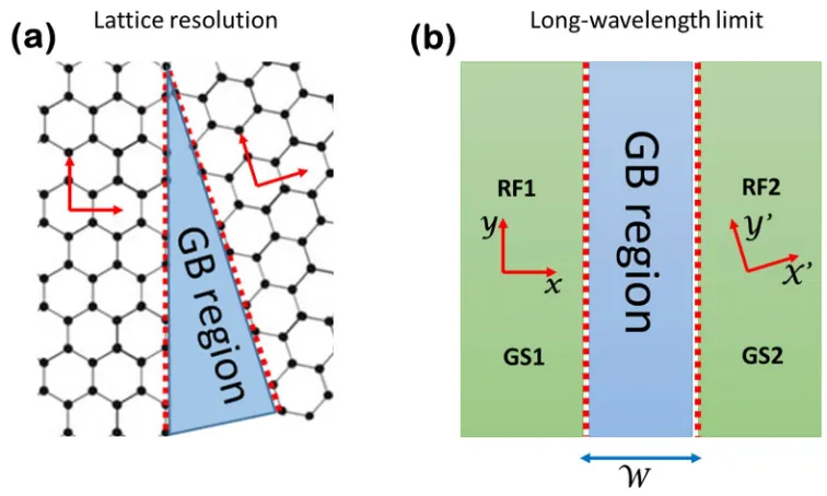
Figure 1. (a) Schematic of the region close to a grain boundary (GB region). Apart from the grain
74
boundary region, where lattice distortions and vacancies affect honeycomb lattice structure of
75
graphene, the bulk of the system is described by a regular atomic arrangement in which the lattice
76
orientation is subject to a rotation of a definite angle going from the left to the right side of the junction.
77
(b) The long-wavelength limit of the grain boundary junction depicted in panel (a). The graphene
78
sheet 1 and 2, namely GS1 and GS2, represent the two sides of the junction, while the GB region is
79
represented by a region of negligible extension W whose effects on the scattering properties of the
80
junction are captured by appropriate boundary conditions. Boundary conditions are direct
81
imposes a lattice rotation of the GS2 compared to the GS1. This effect is easily described using distinct
83
local reference frames, RF1 and RF2, in describing the two sides of the system. Translational
84
invariance along the y-direction of the RF1 is assumed.
85
2. Dirac Hamiltonian within a rotated reference frame, current density conservation and
86
boundary conditions at a grain boundary
87
In this Section we provide a first approach to the grain boundary problem in graphene. We deal
88
with a theory of spinless particles described by the continuous Dirac Hamiltonian and consider a
89
single valley degree of freedom. Neglecting the electron spin is appropriate in the absence of
90
magnetic fields or magnetized regions, which is the case considered in this work. On the other hand,
91
describing graphene electrons adopting a single-valley perspective requires an appropriate
92
justification. Indeed, in principle, grain boundary region can be the source of valley-flipping
93
scattering events. The existence of such kind of phenomena has inspired the emerging field of
94
valleytronics [21] aiming at manipulating the valley degree of freedom as it is done with the spin in
95
spintronics. Valleytronics manipulations, however, require engineered scattering centers, which are
96
quite challenging to implement using current technologies. In view of this circumstance, we can
97
argue that valley-mixing scattering events are quite rare in spontaneously-formed grain boundaries.
98
Moreover, with good approximation, electrons having different valley degree of freedom can be
99
described as two independent quantum fluids. The latter argument justifies the single-valley
100
treatment adopted. Generalization of the ideas exposed hereafter to spinful particles having
two-101
valley degrees of freedom is in principle immediate.
102
2.1. Dirac Hamiltonian within a rotated reference frame
103
In this subsection we describe the continuous Dirac Hamiltonian of a single graphene sheet within a
104
rotated reference frame. Continuous approach considered in this work is appropriate in describing
105
the system conduction properties (e.g., the differential conductance) when the electron wavelegth,
106
associated with the particle momentum, is much longer than the interatomic distance of the
107
honeycomb lattice. While the latter assumption is clearly invalidated in graphene nanoribbons
108
devices, it is appropriate for a large variety of graphene-based devices where micrometric graphene
109
sheets are employed as conduction channels.
110
Let us describe the Dirac Hamiltonian of the graphene sheet GS2, in Fig. 1, in terms of the reference
111
frame of the graphene sheet GS1. The Hamiltonian of GS2 written in terms of RF2 takes the usual
112
form:
113
= 0 ̂ − ̂
̂ + ̂ 0 , (1)
where = ±1 represents the valley quantum number, is the Fermi velocity, while ̂ = − ℏ
114
and ̂ = − ℏ are the quantum mechanical operators associated with the linear momentum
115
components of quasiparticles. The matrix structure of the Hamiltonian originates from the presence
116
of two atoms inside the unit cell of the graphene Bravais lattice. Accordingly the wave function
117
( , ) = ( , ) describing the quantum state of the charge carriers is a two-component spinor
118
whose components are related to the probability of finding the particle on the atom A or B of the unit
119
cell. For the reasons explained above, we neglect the valley quantum number and set = 1. The
120
correspondence between the wave functions expressed in RF1 or RF2 is established observing that
121
the -component of the wave function written in RF1, i.e. ( , ), is related to the homologous
122
component in RF2 by the equation ( , ) = ( , ), ( , ) , with ∈ { , }. The relation
123
= cos sin
−sin cos , (2)
with an appropriate rotation angle. From the above observations one obtains useful relations
125
linking the partial derivatives of the wave functions in the form
126
Φ ( , )
Φ ( , ) =
cos −sin
sin cos
Ψ ( , )
Ψ ( , ) . (3)
Using equation (3) in evaluating the quantity ( , ), one easily get the equality:
127
Ψ( , ) = Φ( , ), (3)
where
128
= 0 ̂ − ̂
̂ + ̂ 0 (4)
represents the Hamiltonian of GS2 written in terms of the RF1. Solving the eigenvalues problem
129
= , with the usual planewave ansatz = ( , ) , one finds eigenstates
130
=
√
1
( ) ⃗ ∙ ⃗, (5)
with associated eigenvalues = ℏ | |. Here = ±1 represents the band index ( = 1 for
131
conduction band and = −1 for valence band), ⃗ = | |( ( ) , ( )) is the particles wavevector
132
and ⃗ = ( , ) is the coordinates vector. The above results show that physical properties of the
133
system, like e.g. the energy spectrum, are reference-frame independent and are clearly reminiscent
134
of the rotational invariance of a bulk (monocristallyne) graphene sheet. Up to now, we have limited
135
our attention to the problem of a single graphene sheet and its description within a rotated reference
136
frame. We have found that the rotated Hamiltonian depends on a phase factor ± , which is not
137
observable. Hereafter we study the junction depicted in Fig. 1, where graphene sheets with different
138
reticular orientations are connected by means of a grain boundary region. Setting the RF1 as a global
139
reference frame, the Hamiltonian of the entire system takes the piecewise form:
140
= → < 0> 0. (6)
The line = 0 defines the grain boundary region in the limit → 0, which is an appropriate
141
approximation when the grain boundary extension along the x-direction is negligible. This
142
requirement is always met by real grain boundaries which are defected regions where covers at
143
least few lattice sites. The latter observation suggests that the scattering properties of the grain
144
boundary region are adequately captured by appropriate boundary conditions within the framework
145
of a continous model. Such boundary conditions are non-standard and are the object of the
146
subsequent analisys. Indeed, when the grain boundary problem formalized so far is treated using
147
ordinary boundary conditions, a violation of the current conservation is found, which is a clear
148
indication that modified boundary conditions are required. Thus, the solution of the problem first
149
requires the derivation of the current density conservation law.
150
151
2.2. Current density conservation
153
Before treating the grain boundary problem, let us consider the current density conservation law
154
originated by the rotated Hamiltonian (4). Continuity equation in the form + ⃗ ∙ ⃗ = 0 is
155
obtained taking the time derivative of the charge density = = | | + | | (the electric
156
charge is omitted) using in the computation the rotated Dirac equation in the form = ( ℏ) .
157
After straitforward computation, current density components, namely = and =
158
, are easily recognized. Here the first quantized current density operators take the following
159
form:
160
= 0
0 (7)
= 0 −
0 , (8)
whose structure explicitely depends on the rotation angle . It is worth mentioning here that the
161
expressions for the = 0 case coincide with the usual relations = and = , where
162
and represent ordinary Pauli matrices. In the following dsicussion, we denote the quantities in
163
equation (7) and (8) as , in order to stress the dependence on the rotation angle , while notation
164
, will be adopted to indicate the same quantities when = 0.
165
2.3. The mathematical problem of boundary conditions at a grain boundary
166
We are now ready to treat the problem of a grain boundary. This situation is schematized using the
167
Hamiltonian model given in equation (6). Accordingly, the current density operator does not admit
168
a global definition, while the following piecewise definition
169
, ( ) =
, < 0
, > 0
(9)
is required. The form of equation (9) fully explains the ultimate reasons of the failure of usual
170
boundary conditions in describing the scattering problem defined by the Hamiltonian in (6).
171
Hereafter, we provide a careful explanation of this point. First of all, we explicitly observe that, under
172
translational invariance along the y-axis, the y-component of the current density, namely =
173
Ψ Ψ, does not depend on the coordinate y and thus the quantity = 0 does not play any role
174
in the continuity equation. Therefore, current density conservation entirely depends on the
175
conservation of the x-component of the current density. The current density conservation problem is
176
related to the invariance of the current density operator under appropriate transformations. This
177
point can be easily understood observing that within the transfer matrix formalism boundary
178
conditions for the spinorial wave function at the = 0 interface can be written as Ψ(0 ) = ℳΨ(0 ),
179
with ℳ a 2 × 2 matching matrix. Here we have introduced the notation 0 and 0 , meaning a
180
spatial position close to = 0 and belonging to the right or left side of the junction, respectively.
181
Within this formalism the current density on the right (left) side of the interface, namely ( ),
182
takes the form = Ψ (0 ) (0 )Ψ(0 ) ( = Ψ (0 ) (0 )Ψ(0 )), while current density
183
conservation requires the condition = . Observing that = Ψ (0 )ℳ (0 )ℳΨ(0 ) and
184
using the continuity of the current density at the interface, we get the important relation
185
ℳ (0 )ℳ = (0 ). Here we explicitly notice that current density operator in the absence of
186
lattice mismatching at the interface (i.e. = 0) is globally defined so that (0 ) = (0 ) and the
187
usual boundary conditions are recovered. This is not the case for the problem under study where
188
(0 ) ≠ (0 ), as evident by direct inspection of equation (9). According to the above arguments,
189
proper boundary conditions for the scattering problem at the grain boundary interface are assigned
190
once an opportune matching matrix ℳ has been identified. Based on the current density
191
conservation law, a matching matrix ℳ have to respect the following matrix equation
192
ℳ ℳ = ⟹ ℳ 0
0 ℳ = (10)
for arbitrary choices of the rotation angle . The matching matrix ℳ is completely determined by
194
the properties of the grain boundary local potential ( ) to be added to the Dirac Hamiltonian (6).
195
Such potential is a 2 × 2 Hermitian operator which is different from zero only inside the grain
196
boundary region (the GB region in Fig. 1 (b)), while its specific form depends on the realization of the
197
interface between grains at atomic level. The latter information is clearly not available within the
198
framework of a long wavelength (continuous) model and thus ( ) have to be meant as a
199
phenomenological potential able to reproduce the transport properties of the interface. A useful
200
simplification which will be used in the following discussion parametrizes the interface potential as
201
( ) = ℬ ( ) with ( ) the Dirac delta function and ℬ a 2 × 2 Hermitian operator. Once the
202
structure of ( ) = ℬ ( ) is known, the matching matrix ℳ can be determined as described in Sec.
203
2.5.
204
An alternative and interesting approach is completely based on the algebraic properties of the
205
matching matrix ℳ. The algebraic method allows the identification of all possible matching matrices
206
in the absence of any information on the scattering potential ( ). The generality of this approach,
207
which will be presented in Sec. 2.4, is quite appealing in describing real systems where precise
208
information on the interface are not available.
209
2.4. Algebraic classification of the matching matrix ℳ for the grain boundary problem
210
In this subsection we study the general problem of a grain boundary formed between two graphene
211
sheets whose reticular axes are rotated by the angles and , respectively. Under this general
212
condition, the grain boundary Dirac Hamiltonian takes the following piecewise form
213
= < 0
> 0. (11)
Moreover, we assume that an unknown grain boundary potential ( ) is present at the interface
214
located in = 0. Our purpose is deriving the general structure of all possible matching matrices ℳ
215
disregarding the unknown properties of the grain boundary potential. First of all, we do observe that
216
current density conservation takes the general form ℳ ℳ = which is insensitive to the
217
transformation ℳ ⟶ ℳ, being an arbitrary phase factor. The latter property will be taken into
218
account in the following presentation by omitting the arbitrary phase factor.
219
In order to follow our program we consider two relevant classes of matching matrices: (i) matching
220
matrices belonging to the special unitary group SU(2) constituted by 2 × 2 unitary matrices with
221
determinant equal to 1; (ii) matching matrices belonging to the special linear group SL(2,C)
222
constituted by 2 × 2 matrices with determinant equal to 1 defined over the complex number field.
223
Let us start with the case of ℳ ∈ SU(2). This class of matching matrices contains the identity matrix
224
ℳ = 1 × which is involved in the matching condition Ψ(0 ) = Ψ(0 ) (continuity of the wave
225
function) used, for instance, in describing Klein tunneling phenomenon through a rectangular
226
electrostatic potential. We solve the matrix equation coming from the current density conservation
227
by substituting the following general parametrization of ℳ ∈ SU(2)
228
ℳ =
( ) ( ) ( ) ( )
− ( ) ( ) ( ) ( ) , (12)
being , , real parameters to be determined. The solution of the matrix equation allows the
229
identification of the unknown parameters which appear in equation (12). After straightforward
230
computation we obtain that a general SU(2) matching matrix takes the form:
231
232
ℳ = ( ) ( )
( ) ( )
As expected, ℳ only depends on the relative angle − ≠ 0 formed by the crystallographic axes
233
of the graphene sheets forming the two sides of the grain boundary junction. Interestingly, ℳ
234
cannot be equal to the identity matrix within the SU(2) parametrization and thus the usual boundary
235
condition Ψ(0 ) = Ψ(0 ) is not compatible with the current density conservation in the presence of
236
a grain boundary. In particular, while off-diagonal contribution in ℳ can be eliminated by setting
237
= 0, diagonal terms are always different from one when − ≠ 0, the latter being the condition
238
of interest in the grain boundary case. Ordinary boundary conditions, namely Ψ(0 ) = Ψ(0 ), are
239
correctly recovered by setting − = 0. Physical meaning of the parameter will be clarified in
240
Sec. 2.5.
241
A similar procedure can be applied to the case of ℳ ∈ SL(2, C), where the unitary condition is relaxed
242
compared to the previous case. Under this assumption, we obtain the following matching matrix
243
parametrizations:
244
ℳ = −
, (14)
with , , , ≥ 0, | − | = 1 and = ( − ). An additional matching matrices set,
245
which cannot be obtained from equation (14) under suitable assumptions, is given by
246
ℳ =
, (15)
with , , , ≥ 0 and + = 1. Interestingly, the only diagonal matching matrix such that ℳ ∈
247
SL(2, C) takes the form ℳ = , , with > 0. Moreover, matching
248
matrices belonging to SL(2, C) admit a three parameters description, while SU(2) parametrization
249
requires only one parameter.
250
The matching matrices ℳ, , define a rather general set of physically relevant matching matrices
251
whose structure is fully defined by algebraic properties which are the direct manifestation of the
252
conservation laws of the problem. The matching matrix parametrizations given in equation (13)-(15)
253
are one of the main results of this work. Physical consequences of the matching matrix structure and
254
of its algebraic properties will be discussed later on.
255
2.5. Direct derivation of the matching matrix ℳ from the scattering potential ( ) = ℬ ( ).
256
In this section we provide a link between the features of the scattering potential ( ) and the
257
parameters , , , , introduced in equation (13)-(15). To follow this program, we set aside the
258
problem of grain boundary for a moment and focus our attention on the scattering problem described
259
by the Hamiltonian = → + ℬ ( ), being ℬ = ℬ an Hermitian operator in the sublattice space.
260
As will be discussed in Sec. 3, this problem is related to the grain boundary problem by a local unitary
261
transformation and thus it is not collateral in our discussion. First of all, we do observe that deriving
262
proper boundary conditions for a Dirac delta potential in Dirac equation requires some care [22].
263
Indeed the usual procedure followed in the case of the Schrödinger equation for massive particles
264
does not work when the quantum operator associated to the particle kinetic energy is represented by
265
a first order derivative with respect to the space variable. Under this circumstance, the particle wave
266
function ( ) is not constrained to be continuous in = 0 (i.e. (0 ) ≠ (0 )) and thus the
267
integral ∫ ( ) ( ) , with > 0, is an illdefined quantity. In priciple, since ( ) = (− ), one
268
may argue that ∫ ( ) ( ) = [ (0 ) + (0 )]/2, but this conclusion is uncorrect and leads to
269
contraddictions. To avoid these difficulties, we provide an alternative derivation. Let us start with
270
the stationary Dirac equation ( , ) = ( , ) , with ( , ) = ( ) due to the
271
translational invariance along the y-direction. Since we are interested in the wave function behavior
272
in close vicinity of = 0, we only retain the diverging potential in the Dirac equation. This procedure
273
leads to the first-order differential equation ( ) = ( ) ( ), with ( ) = − (ℏ ) ( ) ℬ,
274
which time-ordered operators are involved. Similarly, formal solution of our problem involves the
276
definition of a space-ordering operator [⋯ ] instead of the usual time-ordering operator. In
277
particular, formal solution can be derived by integration with the following result:
278
Ψ( ) = Ψ( ) + ∫ ( )Ψ( ) . (16)
Infinite iteration of equation (16) leads to the formal solution ( ) = ∫ ( ) ( ),
279
where the action of the space-ordering operator is defined as [ ( ) ( )] = ( ) ( ) ( −
280
) + ( ) ( ) ( − ), while ( − ) represents the Heaviside step function. An important
281
observation for our derivation is that when the commutator [ ( ), ( )] is a vanishing quantity
282
space ordering simply gives [ ( ) ( )] = ( ) ( ). When the above arguments are applied
283
to our original problem using a limit procedure (i.e., → − and → , with → 0), we
284
immediately get:
285
Ψ(0 ) = (− (ℏ ) ℬ)Ψ(0 ). (17)
Direct inspection of (17) allows us to identify the matching matrix ℳ = (− (ℏ ) ℬ) and its
286
dependence on the scattering potential. In the following we provide relevant examples of matching
287
matrices based on the analysis of equation (17). We use the general parametrization for the Hermitian
288
matrix (ℏ ) ℬ reported below
289
(ℏ ) ℬ = , (18)
being , , and real parameters. Once the scattering potential has been characterized using the
290
parametrization given in (18), the matching matrix can be computed by direct exponentiation of the
291
matrix
292
− (ℏ ) ℬ = − ≡ . (19)
Hereafter, we provide explicit examples of the implementation of this procedure and its outcomes.
293
Case 1: = = and =
294
This case corresponds to consider an interface potential of the form:
295
( ) = ℏ Λ 0
0 Λ ( ). (20)
Following the procedure described before we obtain the matching matrix:
296
ℛ = cos(Λ) − sin(Λ)
− sin(Λ) cos(Λ) , (21)
which is an SU(2) matrix (i.e., (ℛ) = 1 and ℛ ℛ = 1) parametrized by the dimensionless
297
quantity . The comparison of equation (21) with (13) shows that the identification ℛ = ℳ is
298
possible by taking − = and = = 0. The above comparison makes a link between the
299
dimensionless potential amplitude in equation (20) and the parameter , which is the free
300
parameter caming from the algebraic analisys carried out in Sec. 2.4. In this way the physical meaning
301
Case 2: = , = − and = (mass term)
303
This case corresponds to consider a mass term potential of the form:
304
( ) = ℏ Λ 0
0 −Λ ( ). (22)
The matching matrix corresponding to this interface potential takes the form:
305
ℛ = cosh(Λ) sinh(Λ)
− sinh(Λ) cosh(Λ) , (23)
which is not unitary (ℛ ℛ ≠ 1) and belongs to the (2, ), implying that (ℛ) = 1. It is easy to
306
prove that equation (23) can be obtained by properly fixing the free parameters which appear in
307
equation (14).
308
Case 3: = = and =
309
This case corresponds to consider an interface potential of the form:
310
( ) = ℏ 0 Λ
Λ 0 ( ). (24)
Physical meaning of this kind of interface potential is explained in Appendix A; here we just comment
311
that the introduction of an off-diagonal potential in the Dirac equation produces a displacement of
312
the K, K’ points in momentum space, the latter effect being usually the result of lattice deformations,
313
e.g. induced by mechanical strain. The matching matrix corresponding to the interface potential given
314
in (24) takes the form:
315
ℛ = ( ) ( ) 0
0 ( ) , (25)
which is defined by a pure phase factor ( ) multiplied by a determinant one diagonal matrix
316
belonging to (2, ). According to our previous discussion, this kind of matching matrices preserve
317
the current density at the interface and thus they are admissible matching matrices despite the
318
determinant is different from one. A direct proof of this statement is provided here for the sake of
319
completeness. Jacobi formula for a generic complex coefficients square matrix implies that
320
( ( )) = ( ) , being ( ) the trace of . When is substituted with in (19) we get
321
(ℳ) = ( )
, with ℳ = the matching matrix of the problem. In this way, we have
322
proven that the determinant of a matching matrix is fixed to one only for diagonal interface potentials,
323
while it is a pure phase factor when off-diagonal terms affect the structure of the interface potential
324
(i.e., when ≠ 0).
325
3. Grain boundary Hamiltonian model with position-dependent rotation angle ( )
326
Before characterizing the scattering properties of a grain boundary, we would like to understand if a
327
phase gradient alone can generate a non-vanishing scattering potential at the grain boundary
328
junction. To answer this question, we need a convenient model in which the phase profile at the
329
interface is a smooth function of the position. Thus, a regularization of the Hamiltonian model
330
presented in (11) is needed. A regularized Hamiltonian model is obtained by taking the rotation angle
331
as a position-dependent function ( ) defining a smeared step function; it provides a gentle
332
matching between the lattice rotation angle on the left of the junction and , characterizing the
333
right side. In this way, a finite phase gradient is present inside the grain boundary region (i.e. the
334
substitution → ( ) in equation (4). This because, according to quantum mechanics prescriptions,
336
terms like ( ) ̂ have to be symmetrized to avoid non-Hermitian contributions to the
337
Hamiltonian. After the symmetrization procedure has been implemented, the following regularized
338
grain boundary Hamiltonian is obtained:
339
( )=
0 ( ), ̂ − ( ) ̂
( ), ̂ + ( ) ̂ 0 , (26)
where we have introduced the anticommutator , = + between generic quantum
340
operators and . It is easy to demonstrate that the dependence on ( ) in (26) can be eliminated
341
using the local unitary transformation
342
( ) = ( )/ 0
0 ( )/ . (27)
In particular, as anticipated in Sec. 2.5, we obtain ( ) ( ) ( ) = ( ) , the latter result being
343
independent on the specific functional form of ( ). Moreover, terms in the Hamiltonian (26)
344
depending on the phase gradient ( ) are exactly cancelled by the unitary transformation.
345
According to these arguments, the mismatch of the crystallographic axes at the grain boundary of a
346
Dirac material does not provide disturbance for particles transmission, at least in the framework of
347
the present model. This conclusion crucially depends on the first order nature of the differential
348
operator representing the kinetic energy of the Dirac particles.
349
When the Hamiltonian presented in (26) includes a generic interface potential of the form:
350
= ℏ ( ), (28)
the complete Hamiltonian takes the form ( )+ . The application of the unitary transformation
351
(27) now leads to the transformed Hamiltonian problem ( ) ( )+ ( ) = ( ) + ,
352
being the transformed interface potential given by
353
= ℏ
( )
( ) ( ), (29)
with , , and dimensionless real parameters. The transformed potential explicitly
354
contains a dependence on the phase value (0) assumed at the grain boundary position = 0. This
355
behavior is specific of the Dirac Delta potential which is appropriate to describe grain boundary
356
interface in the long wave length limit. Here we notice that, the relation between (0) and ,
357
depends on the details of the ( ) dependence. To be specific, a simple model of ( ) can be
358
expressed, e.g., by the following piecewise function:
359
( ) = ( − )/2 +
> /2
( + )/2 ∈ [− /2, /2]
< − /2
, (30)
according to which (0) = ( + )/2. In equation (30), where the limit → 0 has to be meant, ∈
360
[− , ] represents the grain boundary region. As a final comment, we argue that the scattering
361
problem related to the transformed Hamiltonian ( ) + can be treated using ordinary
362
4. Results of the scattering theory
364
4.1. Transmission properties of a n/n’ grain boundary junction with unconventional boundary conditions
365
Purpose of this section is providing simple examples of use of unconventional matching matrices and
366
create a link between the trasmittance properties of the problem and the specific matching matrix
367
adopted. A complete analysis of all condution regimes of the junction (e.g., the p/n case) is beyond
368
the scopes of this section. Thus, we study the scattering problem of a n/n’ grain boundary junction
369
described by the Hamiltonian (6). The peculiar properties of the trasmittance are derived using
370
matching matrices with simplified structure compared to those described in Sec. 2.4.
371
The scattering states in the left and rigth part of the junction are expanded in terms of local eigenstates
372
taking into account the translational invariance of the scattering region along the y-direction.
373
According to this procedure, the scattering sates, normalized by the absolute value of the group
374
velocity , along the propagation direction, can be written in the following general form:
375
Ψ ( , ) = 1 + ℛ 1
−
Ψ ( , ) = (1 )
. (31)
Here ( , ) describes the reflection of a particle belonging to the conduction band ( > 0)
376
impinging from the left on the grain boundary interface with group velocity = and linear
377
momentum =
ℏ , ∈ [− /2, /2] being the incidence angle formed by the particle
378
trajectory with the x-axis. The expression of is related to the dispersion relation on the left side of
379
the junction, namely = ℏ + , by the usual relation = ℏ . In writing the reflected
380
wave contribution (weighted by the reflection coefficient ℛ) we have explicitely taken into account
381
the fact that the reflection angle is related to the incidence angle by the relation = − . In
382
the rigth part of the junction ( > 0) the wave function ( , ) describes a trasmitted electron with
383
group velocity = and linear momentum =
ℏ . Since we are assuming the
384
alignment of the Dirac points of the left and right part of the junction, the dispersion relation of the
385
transmitted electron is given by = ℏ + . Here is worth mentioning that the spinor of the
386
transmitted particle explicitely depends on the rotation angle characterizing the rotation of the
387
cristallographic axes of the right part of the junction. In the elastic scattering of a translational
388
invariant system along the direction both the energy and the linear momentum along the
y-389
direction are conserved quantities. This observation implies that = . Observing that =
390
ℏ and =ℏ , we conclude that = . Scattering states in (31) are used to derive the
391
scattering problem equation ( = 0, ) = ℳ ( = 0, ), whose structure is fixed once the
392
matching matrix ℳ has been specified. Once the scattering equation have been solved, scattering
393
coefficients ℛ and are determined; moreover, current density conservation implies |ℛ| + | | =
394
1. The transmittance | | is an agle-resolved quantity which is directly related to the scattering
395
properties of the interface and determines the differential conductance of the system. In the following
396
several relevant cases are treated, while the transmittance curves as a function of the incidence angle
397
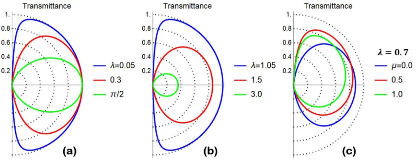
are presented in Figure 2 (a)-(c).
398
Case 1: SU(2) matching matrix (Eq. (13))
399
We have solved the scattering problem using the SU(2) matching matrix given in equation (13) by
400
fixing = 0. The transmittance of the problem has been derived and takes the following (energy
401
| ( )| = ( ) ( ) ( ). (32)
The main property of equation (32) is that | ( = 0)| = 1 for any choice of the parameter (see
403
Fig. 2 (a)). This behavior, which is reminiscent of the Klein tunneling, is clearly inappropriate to
404
describe the grain boundary physics for which a reduction of the transmittance is expected when the
405
strength of the scattering potential (controlled by ) is increased. No dependence on is present in
406
the transmittance since the transmission coefficient ( ) presents an irrelevant prefactor / .
407
Case 2: matching matrix belonging to (2, ); example 1
408
We have solved the scattering problem using the (2, ) matching matrix
409
ℳ = √1 + / − /
/ √1 + / , (33)
which is a special case of the matching matrix given in equation (14) and it is appropriate to describe
410
interface potentials proportional to (mass term). The solution of the scattering problem provides
411
the scattering coefficients:
412
( ) = /
ℛ( ) =
, (34)
implying an angle-independent transmittance given by | ( )| = 1/(1 + ), which is a decreasing
413
function of the scattering strength parameter . This kind of matching matrix seems to be appropriate
414
to describe the conductance reduction induced by a grain boundary region, even though no
415
dependence on is detected. The above findings confirm the confining properties of a potential
416
proportional to .
417
418
Figure 2. (a) Polar plot of the transmittance (transmission probability) | ( )| versus the incidence angle
419
computed according to equation (32) and setting the model parameters as specified in the legend. The matching
420
matrix used belongs to SU(2) and accordingly full transmission is observed for = 0 incidence, the latter result
421
being insensitive to the parameter choice and reminiscent of the Klein tunneling phenomenon. (b) Polar plot of
422
the transmittance (transmission probability) | ( )| versus the incidence angle computed according to
423
equation (36) and setting the model parameters as specified in the legend. Diagonal (2, ) matching
424
matrix (see equation (35)) has been used. A reduction of the transmittance is observed for arbitrary values of
425
| ( )| versus the incidence angle computed according to equation (38) and setting the model parameters
427
as specified in the legend. Non-diagonal (2, ) matching matrix (see equation (37)) has been used. An
428
anisotropic reduction of the transmittance is observed for arbitrary values of the incidence angle as the parameter
429
is increased. Preferential transport directions are obtined.
430
Case 3: matching matrix belonging to (2, ); example 2
431
We have solved the scattering problem using the diagonal (2, ) matching matrix
432
ℳ = / 0
0 / . (35)
The transmittance of the problem has been derived and takes the following (energy independent)
433
form:
434
| ( )| = ( )( ). (36)
A reduction of the transmittance (see Fig. 2 (b)) is observed when the scattering strength parameter
435
is increased, the latter behavior being appropriate to describe the grain boundary physics.
436
Case 4: matching matrix belonging to (2, ); example 3
437
We have solved the scattering problem using the following (2, ) matching matrix
438
ℳ = / − /
0 / , (37)
Which depends on the dimensionless parameters and . The transmittance of the problem has
439
been derived and takes the following (energy independent) form:
440
| ( )| = ( )
[ ( ) ( ) ]. (38)
A reduction of the transmittance is observed when the scattering strength parameter is increased,
441
the latter behavior being appropriate to describe the grain boundary physics. Moreover, depending
442
on the choice of parameters, preferential transport directions are obtained (see Fig. 2 (c)).
443
The analysis of the cases 1-4 shows that the grain boundary transmittance can be independent on ,
444
despite the matching matrix and the spinorial wave function (see equation (31)) present a dependence
445
on this parameter. Furthermore, direct computation (not reported here) shows that -independent
446
trasmittance is not a peculiarity of the single barrier case, but survives in the double barrier case even
447
when the different regions of the conduction channel are described by Dirac Hamiltonian rotated by
448
different angles. The above behavior suggests that the algebraic deduction of the matching matrix
449
structure (see Sec. 2.4) is not able to capture hidden dependence on the rotation angle , which in
450
principle can be important.
451
To clarify this point, in the subsequent section, we analyze a simple model of n/n’ grain boundary
452
junction based on the Hamiltonian treatment proposed in Sec. 3. The physical conditions under which
453
the system presents a -dependent differential conductance are studied.
454
455
4.2. Grain boundary junction with -dependent differential conductance
457
We now formulate a theory of the n/n’ grain boundary junction based on the Hamiltonian model
458
presented in Sec. 3. Let us consider the grain boundary junction described by the Hamiltonian
459
= ( )+ ( ) + ( ), where ( ) is the interface potential introduced in equation (28), while
460
( ) is a step-like potential
461
( ) = 0 < 0
× > 0, (39)
mimicking a potential profile induced by charge transfer at the grain boundary. Such potential is
462
assumed to be diagonal in the sublattice representation, × = (1,1) representing the identity
463
in the sublattice space. Using unitary transformation (27) the Hamiltonian problem can be written in
464
the equivalent form ( ) ( )+ ( ) + ( ) ( ) = ( ) + ( ) + ( ) ≡ ℋ, where ( )
465
is given in (29), while ( ) is invariant under unitary transformation. The junction described by ℋ
466
can be treated using ordinary boundary conditions which are implemented using the matching
467
matrix formulation given in Section 2.5. Since we are interested in verifying the existence of
468
preferential transport directions, we focus our analysis on the interface potential
469
( ) = ℏ
( )
( ) 0 ( ), (40)
which is obtained from equation (29) by setting = 0. The matching matrix associated to (40) is
470
given by
471
ℳ =
ℊ 0
( ) ℊ ℊ∗
( ) ℊ
∗ , (41)
which defines a (2, ) boundary condition with parameters ℊ = ( ), ℊ∗= ( ) and
472
= . Equation (41) presents an explicit dependence on the rotation angle (0) at the grain
473
boundary junction and thus a dependence of the transport properties of the system on this parameter
474
is expected.
475
476
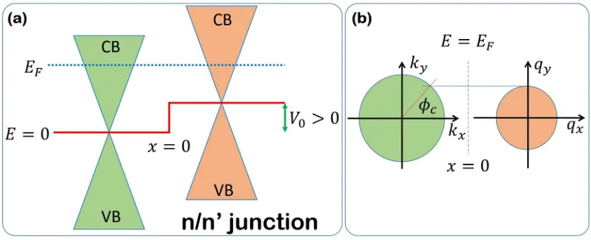
Figure 3. (a) Bands alignment of the n/n’ junction model considered in the main text. Grain boundary interface
477
is located in = 0. The system Fermi level is located above the Dirac points and thus n-type conduction regime
478
is established. (b) In translational invariant system along the y-direction the corresponding linear momentum is
479
angle , y-component of the linear momentum cannot be conserved and no current can flow through the
481
interface.
482
In order to present the results of the model, we focus our attention on the n/n’ junction described in
483
Fig. 3 (a)-(b). The scattering problem related to the conduction properties of the junction is solved
484
using scattering states given in (31) with = 0. However, differently from the case treated in Section
485
4.1 dispersion relation in distinct sides of the junction, namely ( / ), are different and in particular
486
we have that ( )= ℏ + = ℏ | | for < 0 and ( )= ℏ + + = ℏ | | +
487
for > 0. The group velocities are the same considered before and remain unaffected by the presence
488
of a potential step at the interface. Energy of a particle is conserved during the scattering event
489
and thus we can set ( )= ( )= . The latter relation allow us to deduce the moduli of the linear
490
momenta on the different junction sides, namely | | = /ℏ and | | = ( − )/ℏ with −
491
> 0 since we are considering an n/n’ junction. The y-component of the linear momentum on
492
different sides of the junction is thus given by = | | and = | | , while translational
493
invariance implies = . Conservation of the y-component of the linear momentum implies the
494
following relation between the incidence and the transmission angle:
495
= sin sin . (42)
Since the quantity > 1, there exists a critical angle of incidence for which equation (42) cannot
496
be satisfied and no current can flow through the interface. Such critical value takes the following
497
form:
498
= sin . (43)
Once the scattering problem has been solved using the matching matrix given in (41) the
angle-499
resolved transmittance | ( )| is derived. The zero-temperature differential conductance of the
500
junction is related to the transmittance evaluated at the Fermi level, = , by the following
501
relation:
502
= ℒ ∫ [| ( )| cos ] , (44)
with = 4 a degeneracy factor caming from the spin ( = 2) and the valley ( = 2)
503
degeneracy, ℒ the transverse dimension of the junction assumed to be a macroscopic quantity and
504
= /(ℏ ) the modulus of the Fermi wave vector. Here is worth mentioning that the Fermi level
505
can be tuned by using a back gate with the twofold effect of modulating the number of transverse
506
channels ( ) = ℒ involved in the conduction and changing the value of the critical angle
507
509
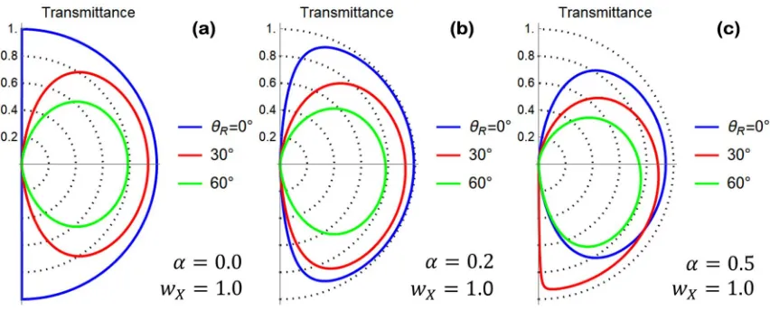
Figure 4. (a) Polar plot of the Transmittance computed according to equation (45) by setting the model
510
parameters as shown in the figure legend. Preferential transport directions are absent, while transmission
511
probability is reduced as the misorientation angle is increased. (b) Polar plot of the Transmittance computed
512
according to equation (45) by setting = 0.2 and = 1. Preferential transport directions are observed. (c)
513
Polar plot of the Transmittance computed according to equation (45) by setting = 0.5 and = 1. Preferential
514
transport directions are observed.
515
Before treating the general case of ≠ 0, we study the solution of the scattering problem under the
516
simplifying assumption = 0, which allow us to obtain the following simple expression for the
517
angle-resolved transmittance:
518
| ( )| =
( ( )) ( ( ))[ ( )] . (45)
Direct inspection of equation (45) evidences a dependence on (0), which is the relic of the
519
cristallographic axes mismatching between the two sides of the grain boundary junction. In the
520
following analysis we use the model for ( ) given in equation (30) with = 0. Accordingly, we
521
set (0) = /2. Furthermore, the analysis of the formation energy of a graphene grain boundary as
522
a function of the misorientation angle shows an M-shaped behavior with a local minimum at
523
≅ 30° and absolute minima in ≅ 0° and ≅ 60° [19]. In Fig. 4 (a)-(c) we have studied the
524
behavior of equation (45) as a function of the relevant junction parameters. A reduction of the
525
transmission probability is observed as the misorientation angle at the grain boundary is
526
increased. Preferential transport directions are clearly related to a non-vanishing value of the
527
parameter .
528
Figure 5. Polar plot of the transmittance of the n/n’ junction computed setting the interface parameters as =
530
0.2 and = 1.0. Different curves in each panel refer to different misorientation angles as indicated in the
531
figure legend. The potential step has been fixed as = 0.1, 0.3, 0.5 in panels (a), (b) and (c), respectively. Due
532
to the critical angle reduction for increasing values of , a suppression of the junction transmission at high
533
incidence angles is clearly visible.
534
The general expression of the transmittance pertaining to the ≠ 0 case is quite lengthy and thus
535
we only present numerical evaluation of it. This analysis is performed in Fig. 5 (a)-(c), where the effect
536
on the transmittance of a finite potential step at the interface is presented setting the values of the
537
remaining junction parameters as done in Fig. 4 (b). Here we observe that the critical angle of the
538
scattering problem is an energy-sensitive quantity which is reduced when the potential step intensity
539
is increased. Figures 5 clearly show the effect of the critical angle reduction and suppression of the
540
junction transmission at high incidence angles is clearly visible.
541
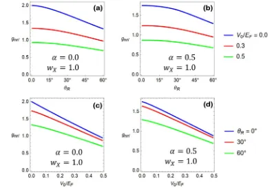
In Fig. 6 (a)-(d) we report the differential conductance given in equation (44) normalized to the
542
quantity ℒ ≡ , the resulting dimensionless quantity being = / . In particular,
543
in Fig. 6 (a)-(b) we show as a function of the misorientation angle for different values of the
544
potential step and of the matching matrix parameters. A suppression of the junction conductance as
545
a function of is observed, the latter behavior being more pronounced for small values of the
546
potential step intensity.
547
In Fig. 6 (c)-(d) we show as a function of the potential step intensity . Different curves are
548
related with distinct choices of the misoriantation angle of the grain boundary junction. An almost
549
linear lowering of the versus curves is obtained which is related to the critical angle
550
reduction causing the progressive closure of the conduction channels.
551
The general conclusion associated to the analysis performed in Figure 6 is that grain boundary
552
junctions with large misorietation angles manifest the tendency to be more opaque compared to those
553
with a better lattice matching. Moreover, charge transfer at the grain boundary interface induces a
554
potential step whose effect is relevant in determining the transparency of the interface.
555
Figure 6. (a), (b) Dimensionless differential conductance as a function of the misorientation angle .
557
Different curves pertain to different values of the intensity of the potential step as indicated in the figures legend.
558
Matching matrix parameters = 0 and = 0.5 are used in the computation of panel (a) and (b), respectively.
559
(c), (d) Dimensionless differential conductance as a function of the potential step intensity . Different
560
curves pertain to different values of the misorientation angle as indicated in the figures legend. Panel (c) is
561
obtained by fixing = 0, while panel (d) is obtained by fixing = 0.5.
562
5. Conclusions
563
We have proposed a continuous model to study grain boundary effects in graphene. The model
564
provides a description of the grain boundary based on Dirac Hamiltonian written in a rotated
side-565
dependent reference frame describing crystallographic axes mismatching at a grain boundary
566
junction. We have shown that the scattering problem related to the transmission properties of a grain
567
boundary junction requires modified boundary conditions, which can be implemented by using the
568
matching matrix method in the scattering problem. We have characterized the algebraic properties
569
of all possible matching matrices showing that SU(2) and SL(2, C) matching matrices are admissible.
570
In particular, we have proven that SU(2) matching matrices support Klein tunneling and are not
571
adequate in describing the conductance lowering associated to a grain boundary physics, which is
572
instead captured by SL(2,C) matching matrices. We have studied specific matching matrix examples
573
and the associated transmittance properties. It has been demonstrated that, under opportune
574
assumptions, preferential transport directions are supported by the interface microscopic properties,
575
which are encoded in our approach by the matching matrix structure.
576
Moreover, using a space-dependent unitary transformation, we have formulated a grain boundary
577
model where usual boundary conditions can be used. Conditions to observe scattering properties
578
related to the crystallographic axes mismatching at the grain boundary interface are studied.
579
Reduction of the junction conductance has been demonstrated as the effect of the misorientation agle
580
between the two junction sides.
581
The proposed theory provides a phenomenological model to study grain boundary physics within
582
the scattering approach and represents per se an important enrichment of the scattering theory of
583
graphene having the potential to stimulate new experiments and further theoretical investigations.
584
585
Acknowledgments: The author acknowledges fruitful discussions with Antonio Troisi on the arguments of this
586
work.
587
Author Contributions: F.R. conceived the idea of this work, developed the theory, its numerical implementation
588
and wrote the paper. A. D. B. contributed in discussing the experimental implications of the theory and to the
589
writing of the manuscript.
590
Conflicts of Interest: The authors declare no conflict of interest.
591
Appendix A
592
Let us consider the rotated Dirac Hamiltonian presented in (4) complemented by the
off-593
diagonal potential in the sublattice space = . The resulting Hamiltonian in momentum space
594
takes the form
595
( ) = ( ) + = ℏ 0 −
+ 0 +
0
0 . (A1)
The spectrum of the problem is obtained by solving the equation [ ( ) − ] = 0 with respect
596
to . Straightforward computation shows that the dispersion relations of the conduction and valence
597
bands take the following form:
598
which clearly shows a dependence on the rotation angle which is absent when the off-diagonal
599
potential is switched off ( = 0). Moreover, the Dirac point, which is defined as the point in the
600
momentum space where = , is displaced from the original K point in momentum space by the
601
vector = −
ℏ , ℏ . In real systems, Dirac cone displacement from the unperturbed K point
602
is related to strain-induced change in the graphene electronic structure [23]. Since grain boundary
603
regions present defective lattice accompanied by mechanical deformations, the off-diagonal potential
604
introduced in (A1) can well emulate strain-induced modifications of the electronic properties.
605
Clearly, in modeling these effects non-vanishing off-diagonal potential is only admissible in close
606
vicinity of the grain boundary region, while it is expected to be irrelevant when an ordered (without
607
defects and vacancies) graphene lattice is restored. The dependence of the spectrum in (A2) on the
608
rotation angle is induced by the properties of the Hamiltonian under unitary transformations.
609
Indeed, rotated Hamiltonian ( ) is unitarily equivalent to the ordinary graphene Hamiltonian
610
according to the relation ( ) = ( ) with
611
= / 0
0 / . (A3)
Accordingly, the spectrum of ( ) does not depend on . The same conclusion is valid in the
612
presence of a diagonal potential. To demonstrate this point, let us apply the same argument to the
613
Hamiltonian = ( ) + , with
614
= 0 0 . (A4)
We observe that the transformed Hamiltonian takes the form = ( ) + since is
615
invariant under unitary transformation, i.e. = . The above observation implies that the
616
energy spectrum remains insensitive to the rotation angle even in the presence of a diagonal
single-617
particle potential .
618
On the other hand, when the above procedure is applied to the Hamiltonian ( ) = ( ) +
619
considered in (A1), we obtain ( ) = ( ) + with
620
= 0
0 , (A5)
the latter being the transformed potential. Since retains a dependence on the rotation angle, a
621
-dependent energy spectrum is obtained for the Hamiltonian in (A1). The above results suggest that
622
the relative angle formed by the crystallographic axes of the two sides of a grain boundary junction
623
can affect the scattering properties of the system in the presence of an off-diagonal potential in the
624
sublattice indices. This conclusion is clearly supported by the arguments presented in Sec. 4.2.
625
References
626
1. Das Sarma, S.; Adam, S.; Hwang, E. H.; Rossi, E. Electronic transport in two-dimensional graphene.
627
Reviews of Modern Physics 2011, 83, 407–470, doi:10.1103/RevModPhys.83.407.
628
2. Allain, P. E.; Fuchs, J. N. Klein tunneling in graphene: optics with massless electrons. The European Physical
629
Journal B 2011, 83, 301–317, doi:10.1140/epjb/e2011-20351-3.
630
3. Rusin, T. M.; Zawadzki, W. Zitterbewegung of electrons in graphene in a magnetic field. Physical Review
631
B 2008, 78, doi:10.1103/PhysRevB.78.125419.
632
4. Tikhonenko, F. V.; Kozikov, A. A.; Savchenko, A. K.; Gorbachev, R. V. Transition between Electron
633
Localization and Antilocalization in Graphene. Physical Review Letters 2009, 103,
634
doi:10.1103/PhysRevLett.103.226801.
635
5. Ostrovsky, P. M.; Gornyi, I. V.; Mirlin, A. D. Theory of anomalous quantum Hall effects in graphene.
636
Physical Review B 2008, 77, doi:10.1103/PhysRevB.77.195430.
637
6. Cheianov, V. V.; Fal’ko, V.; Altshuler, B. L. The Focusing of Electron Flow and a Veselago Lens in