Single Channel Adaptive Kalman Filtering – Based Speech Enhancement Algorithm

(1)

ISSN (Print) : 2320 – 3765 ISSN (Online): 2278 – 8875

I

nternational

J

ournal of

A

dvanced

R

esearch in

E

lectrical,

E

lectronics and

I

nstrumentation

E

ngineering

(An ISO 3297: 2007 Certified Organization)

Vol. 4, Issue 4, April 2015

Single Channel Adaptive Kalman Filtering –

Based Speech Enhancement Algorithm

Prof. M.V. Ramanaiah

1

, N. Sirisha

2

, P. Ravali

3

, B. Vinay Singh

4

, T. Thirupathi

5

Professor, Dept of ECE,

MLR Institute of Technology, Dundigal, Hyderabad, TS, India1

UG Students, Dept of ECE,

MLR Institute of Technology, Dundigal, Hyderabad, TS, India2,3,4,5

ABSTRACT: This paper deals with the problem of speech enhancement when a corrupted speech signal with an additive Gaussian white noise is the only information available for processing. Speech enhancement aims to improve speech quality by using various algorithms. The objective of enhancement is improvement in intelligibility and/or overall perceptual quality of degraded speech signal using audio signal processing techniques. Enhancing of speech degraded by noise, or noise reduction, is the most important field of speech enhancement. Kalman filtering is known as an effective speech enhancement technique, in which speech signal is usually modeled as autoregressive (AR) process and represented in the state-space domain. Kalman filter based approaches proposed in the past, operate in two steps: they first estimate the noise and the driving variances and parameters of the signal model, then estimate the speech signal. Kalman filtering arise some drawbacks. we need to modify the conventional Kalman filter algorithm. Conventional Kalman filter algorithm needs to calculate the parameters of AR(auto=regressive model), and perform a lot of matrix operations, which is generally called as non adaptive. In this paper we provide a alternate solution that avoids explicit estimation of noise and driving process variances by estimating the optimal kalman gain. It eliminates the matrix operations and reduces the computational complexity and we design a coefficient factor for adaptive filtering, to automatically amend the estimation of environmental noise by the observation data. Experimental results shows that the proposed technique is effective for speech enhancement compare to conventional Kalman filter.

KEYWORDS: Speech enhancement, noise reduction, a priori Signal-to-Noise Ratio, a posteriori Signal-to-Noise Ratio, harmonic regeneration, two step noise reduction

I .INTRODUCTION

(2)

I

nternational

J

ournal of

A

dvanced

R

esearch in

E

lectrical,

E

lectronics and

I

nstrumentation

E

ngineering

II. FILTERING TECHNIQUES FOR SPEECH ENHANCEMENT A. SPECTRAL SUBTRACTION

spectral subtraction is a method for restoration of the power spectrum or the magnitude spectrum of a signal observed in additive noise, through subtraction of an estimate of the average noise spectrum from the noisy signal spectrum. The noise spectrum is usually estimated, and updated, from the periods when the signal is absent and only the noise is present. The assumption is that the noise is a stationary or a slowly varying process, and that the noise spectrum does not change significantly in between the update periods. For restoration of time-domain signals, an estimate of the instantaneous magnitude spectrum is combined with the phase of the noisy signal, and then transformed via an inverse discrete Fourier transform to the time domain. The noisy signal model in the time domain is given by

y n

( )



x n

( ) v(n)



(1)

where y(n),x(n)and v(n) are the signal, the additive noise and the noisy signal respectively, and nis the discrete time index. In the frequency domain , the noisy signal model of Equation 1 is expressed as

Y(f)



X

(f)



V

(f)

(2)

Where Y(f), X(f) and V(f) are the Fourier transforms of the noisy signal

v(n)

y

(n)

,the original signal

x(n)

and the noise

v(n)

respectively, and f is the frequency variable. In spectral subtraction, the incoming signal

x(n)

is buffered and divided into segments of N samples length. Each segment is windowed, using a Hanning, Hamming or Kaiser window, and then transformed via discrete Fourier transform (DFT) to N spectral samples. The windowing operation can be expressed in the frequency domain as

X

_w

( )

f



W f

( ) * Y(f)

(3)

where the operator * denotes convolution. The equation describing spectral subtraction may be expressed as

y k

 



Hx k

   



n k

(4) where



|

X f

( ) |

b is an estimate of the original signal spectrum|

| Y(f) |

b and

| V(f) |

b is the time-averaged noise spectra. It is assumed that the noise is a wide-sense stationary random process. For magnitude spectral subtraction, the exponent b=1, and for power spectral subtraction, b=2. The parameter α in Equation (4) controls the amount of noise subtracted from the noisy signal. For full noise subtraction, α=1 and for over-subtraction α>1.The time averaged noise spectrum is obtained from the periods when the signal is absent and only the noise is present as

1 0

1 | V(f) |

|

( ) |

K

b b

i i

V f

K







(5)

In Equation (5), |Vi(f)| is the spectrum of the ith noise frame, and it is assumed that there are K frames in a noise-only period, where K is a variable. For restoration of a time-domain signal, the magnitude spectrum estimate | Xˆ ( f)|is combined with the phase of the noisy signal, and then transformed into the time domain via the inverse discrete Fourier transform as



2 1

(K) 0

( )

| ( ) |

y

N _j _Kn

j _N

K

x n

x k

e

 

 _





(6)

(3)

I

nternational

J

ournal of

A

dvanced

R

esearch in

E

lectrical,

E

lectronics and

I

nstrumentation

E

ngineering



[|

( ) |]

{|

( ) | if |

( ) |

| Y(f) |

[| ( ) |]otherwise

T X f

X f

fn Y f







(7)

Spectral subtraction may be implemented in the power or the magnitude spectral domains. The two methods are similar, although theoretically they result in somewhat different expected

B.WIENER FILTERING

The wiener filter was proposed by Norbert Wiener in 1940.It was published in 1949. Its purpose is to reduce the amount of noise in a signal. This is done by comparing the received signal with a estimation of a desired noiseless signal. Wiener filter is not an adaptive filter, as it assumes input to be stationary. The aim of the process is to have minimum mean square error. In signal processing, the Wiener filter is a filter used to produce an estimate of a desired or target random process by linear time-invariant filtering an observed noisy process, assuming known stationary signal and noise spectra, and additive noise.

The Wiener filter is similar to Spectral Subtraction in the way it is derived and attempts to minimize the mean-square error in the frequency domain, A noisy signal

s

(n)

can be expressed as

S

(n)



x(n)



y(n)

(8)

Here

x(n)

is the clean speech signal and

y(n)

is the additive noise signal. This same equation in the frequency domain now becomes

(f)

X( ) Y( )

S



f



f

(9)

Where

X( )

f

is the signal spectrum,

Y( )

f

is the noise spectrum. The Wiener filter is written as

(f)

_XX

( ) (P ( )

_XX _YY

(f))

W



P

f



P

(10)

Where

P

_XX

( )

f

the signal is power spectrum and

P

_YY

(f)

is the noise power spectrum. Taking this equation and

dividing top and bottom by

P

_YY

(f)

and letting

(f)

SNR(f) / (SNR(f) 1)

W





(11)

This Equation gives us an important insight into how noise reduction systems work by using a function of the estimates of the SNR ratios to change the spectral amplitudes of signals disrupted with noise. Wiener filtering is not applicable for continuous speech signals. For the quality of speech SNR still needs to be improved.

C.KALMAN FILTERING

The use of Kalman Filter for speech enhancement in the form that is presented here was first introduced by Paliwal (1987). This method however is best suitable for reduction of white noise to comply with Kalman assumption. In deriving Kalman equations it normally assumed that the process noise (the additive noise that is observed in the observation vector) is uncorrelated and has a normal distribution. This assumption leads to whiteness character of this noise. There are, however, different methods developed to fit the Kalman approach to colored noises.

It is assumed that speech signal is stationary during each frame, that is, the AR model of speech remains the same across the segment. To fit the one-dimensional speech signal to the state space model of Kalman filter we introduce the state vector as: equation (13)

(n) [ (n

1) (n

2) (n

3).. (n)]

T

x



x

 

p

x

 

p

x

 

p

x

₍₁₃₎

where x(n) is the speech signal at time n. Speech signal is contaminated by additive white noise N(n):

y

(n)



x

(n)



N

(n)

(14)

The speech signal could be modelled with an AR process of order p.

X k

( )





a x k i

_i

(

 

)

u k i

( );



1...

p

(15)

where ai's are AR (LP) coefficients and u(k) is the prediction error which is assumed to have a normal distribution

(4)

I

nternational

J

ournal of

A

dvanced

R

esearch in

E

lectrical,

E

lectronics and

I

nstrumentation

E

ngineering

x k

( )



Ax k

(

 

1)

Gu k

( )

(16) where,

G



[00



01]

T

A=

1 1

0

1

0

1

0

p p

a

_

a



































G has a length of p (LP order) and the observation equation would be:

 

   

y k



Hx k



n k

(17) where,H=GT

The Kalman filter, like other recursive methods, uses all the series history but with one advantage: it tries to estimate a stochastic path of the coefficients instead of a deterministic one. In this way it solves the possible estimation cut when structural changes happen. The Kalman filter uses the least square method to recursively generate a state estimator on k moment, which is unbiased minimum and variance linear. This filter is in equal terms with Gauss-Markov theorem and this gives to Kalman filter its enormous power to solve a wide range of problems on statistic inference. The filter is distinguished by its skill to predict the state of a model in the past, present and future, although the exact nature of the modeled system is unknown. Among the filter disadvantages we can find that it is necessary to knowthe initial conditions of the mean and variance state vector to start the recursive algorithm. There is no general consent over the way of determinate the initial conditions. When it is developed for autoregressive models, the results are conditioned to the past information of the variable under study. In this sense the prognostic of the series over the time represents the inertia that the system actually has and they are efficient just for short time term.

III .ADAPTIVE KALMAN FILTERING

Gabrea and O'Shaughnessy have proposed estimating the noise and driving process variances using the property of the innovation sequence, obtained after a preliminary Kalman filtering with an initial gain. In this paper the signal is modeled as an AR process and a Kalman filter based-method is proposed by reformulating and adapting the approach proposed for control applications by Carew and Belanger .This method avoids the explicit estimation of noise and driving process variances by estimating the optimal Kalman gain. After a preliminary Kalman filtering with an initial sub-optimal gain, an iterative procedure is derived to estimate the optimal Kalman gain using the property of the innovation sequence. The performance of this algorithm is compared to the one of alternative speech enhancement algorithms based on the Kalman filtering. A distinct advantage of the proposed algorithm is that a VAD(voice activity detector) is not required. Another advantage of this algorithm compared to the one, similar in structure, presented in [8], is the superiority in terms of computational load. A filtering step is not required in the optimal Kalman gain estimation.

A. NOISY SPEECH MODEL AND KALMAN FILTERING The speech signal

s

(n)

is modeled as a pth-order order AR process

1

(n)

(n) s(n

)

u(n)

p i i

s

a

i





 

(18)

y

(n)



s(n) v(n)



₍₁₉₎

Where s(n) is the nth sample of the speech signal, y(n) is the nth sample of the observation, and

a

_i

(n)

is the ith AR parameter.

This system can be represented by the following state-space model:

x

(n)



F(n) x(n 1) Gu(n)

 

₍₂₀₎

(5)

I

nternational

J

ournal of

A

dvanced

R

esearch in

E

lectrical,

E

lectronics and

I

nstrumentation

E

ngineering

(n)

Hx(n) v(n)

y





₍₂₁₎

Where:

1. The sequence

u(n)

and

v(n)

are uncorrelated Gaussian white noise with zero means and the variables

2 2

u

and

v



2.

x

(n)

is the

p



1

state vector

( )

[ (

1)

( )]

T

x n



s n

 

p



s n

(22)

3. F is the

p p



transition matrix

1 2 1

0

1

0

1

0

1

p p p

F

a

_

a

_

a













































4. G and H are, respectively, the

p



1

input vector and the

1 

p

observation row vector which is defined as follows

H



G

T



[0

0 

0 1]

The standard Kalman filter [24] [25] provides the up-dating state vector estimator equations:

( )

( ) H ( /

1)

e n

y n

x n n







(23)

( / )

( /

1)

K(n) e(n)

x n n

 



 

(24)

(

1/ )

( / )

x n

n

F x n n

 





(25)

Where

x n n

( /

1)





is the minimum mean-square estimate of the state vector

x n

( )

given the past observations

(1),

, (

1), ( / )

y

y n

x n n







is the filtered estimate of the state vector

x n

( )

,

e(n)

is the innovation sequence and

K(n)

is the Kalman gain. The estimated speech signal can be retrieved from the state-vector estimator:

s n

( )

H x n n

( / )

 



(26) The noise variances



_u2

and



_v2are needed to compute the Kalman gain

K(n)

. However, the transition matrix and the Kalman gain are unknown and hence must be estimated. The parameter estimation (the transition matrix and the optimal Kalman gain) is presented in the next section.

B. ESTIMATION OF TRANSITION MATRIX

(6)

I

nternational

J

ournal of

A

dvanced

R

esearch in

E

lectrical,

E

lectronics and

I

nstrumentation

E

ngineering

In our approach, getting F requires the AR parameter estimation. This issue being outside the scope of the present paper we propose to estimate the AR parameters from modified Yule-Walker equations [26], even if this approach may sometimes lead to unsatisfactory performances, especially for wideband signals [27]:

†

1

(1)

( )

(

1)

(

1)

(2

1)

(2

1)

p yy yy yy

yy yy yy

a

r

p

r

p

r

p

r

p l

r

p

a

 

  









  







  

_

_



_

_

  

_

_{ }





_



  







 











(27)

Where

r

_yy

( )

k



E

[y( ) y(n k)]

n



denotes the observation autocorrelation function,

E

[.]

denotes the expectation, †

[.]

denotes the pseudo inverse operator and

l



0

C. ESTIMATION OF THE OPTIMAL GAIN

It is known that in the optimal case the innovation process is orthogonal to all past observations

y

(1),



, (

y n



1)

and it consists of a sequence of random variables that are orthogonal to each other. In this case the autocorrelation of the

innovation process

r k

ee

( )



E e n e n k

[ ( ) (



)]

is zero for

k



0

.Let a sub-optimal Kalman gain

K



,

x n n



( /



1)

the estimate of the state vector

x n

( )

given the past observation

y

(1),



, (

y n



1)

and

( )

( /

1)

e n





y n



Hx n n





the innovation sequence obtained using the Kalman gain

K

. In this case the innovation sequence

e n



( )

is not a white process and

r

_ee

( )

k



E e n e n

[ ( ) (

 



k

)]

is not zero for

k



0

. Let define the difference estimate vector

x n n

( /



1)

obtained by difference between the estimates of

x n

( )

using the optimal and respectively the sub-optimal Kalman gain and

M n n

( /

 

1)

E x n n

[ ( /



1)

x n n

T

( /



1)]

and the difference estimate correlation matrix. In the steady-state

K n

( ) ~ K

and

M n n

( /



1) ~

M

Using the estimation transition matrix

F



, the standard Kalman filter equations (8)-(10) and the state space model equations (3)(4), the innovation

autocorrelation function

r

_ee

( )

k

is computed as:

r

ee

H F I

[ (

K H

)]

k 1

F

[(

I

K H MH

)

T

(

K

K r

)

ee

(0)]

 



_

_

 

_

_



_

_



K>0 (28)

r

_ee

(0)



HMH

T



r

_ee

(0)

(29) Using the equation (28), the optimal steady-state Kalman gain is obtained as

1 1 1

(1)

(2)

[ (

)]

(

)

/

(0)

/

(0)

(p)

[ (

)]

ee T ee ee ee ee p

H F

_r

r

H F I

K H

F

K

I

K H MH

r

H F I

K H

F

     _        

































 





























_









(30)

Using the steady-state Riccati equation [24] the difference estimate correlation matrix is obtained as:

* *

(

)

(

)

(0)(

)(K K )

T

T T

ee

M

F I

K H M I

K H

F

r

K

 

 









(31)

(7)

I

nternational

J

ournal of

A

dvanced

R

esearch in

E

lectrical,

E

lectronics and

I

nstrumentation

E

ngineering

Carew and Belanger have proposed an iterative method to solve the equations (29)(30)(31) in terms of

r

_ee

(0)

, K and M. Adapting this method in our case, in the first iteration we start with

M

(0) the initial value of M, compute the first estimates of innovation autocorrelation

r

_ee(0)

(0)

using (29) and compute the first estimate of the optimal Kalman gain

(0)

K

using (30). After I iterations the estimates of

r

_ee

(0)

, K and M are:

( ) (0)

(0)

HM

i T

ee ee

r



r





H

(32)

1 1 ( )

1

(1)

(2)

[ (

)]

(

)

/

(0)

/

(0)

(p)

[ (

)]

ee

i T ee

ee ee

ee p

H F

_r

r

H F I

K H

F

K

I

K H MH

r

H F I

K H

F

 



  _



 



 

 

































 





_

_























_









(33)

( 1) ( ) * ( ) * *

(I K

)

(

)

(0)(

)(K K )

T

i i T i T

ee

M

F

H M

I

K H

F

r

K

 



_

_



_

_

_

(34)

IV .SIMULATION RESULTS

The approach was tested using a speech signal with an additive Gaussian white noise. The speech signals are the sentences from a noisy speech corpus(NOICEUS) data base. The sentences were originally sampled at 25Khz and down sampled at 8Khz.The following signal represent a original speech signal recorded at the gain of 15dB.

Fig.1.Original speech

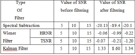
We observed the following estimated speech signal after filtering by using Spectral subtraction method, Wiener filtering (TSNR: Two Step Noise Reduction & HRNR: Harmonic Regeneration Noise Reduction ) and Adaptive Kalman filtering having improvement in the SNR values ,which indicates the quality of voice. After comparison of the outputs of three kind of filters we observed that Kalman provides best quality of speech.

(8)

I

nternational

J

ournal of

A

dvanced

R

esearch in

E

lectrical,

E

lectronics and

I

nstrumentation

E

ngineering

Fig.2. Estimated speech using TSNR

Fig.3. Estimated speech using HRNR

Fig.4.Estimated speech using Adaptive Kalman Filter

The following table shows the output SNR of three types of filters for an input speech signal at different gain levels.

(9)

I

nternational

J

ournal of

A

dvanced

R

esearch in

E

lectrical,

E

lectronics and

I

nstrumentation

E

ngineering

Fig.5.Histogram REFERENCES

[1]: Saeed V. Vaseghi „Advanced Digital Signal Processing and Noise Reduction‟ Third Edition (2005)

[2]: Joachim Thiemann: „Acoustic Noise Suppression for Speech Signals using Auditory Masking Effects‟ „http://www-mmsp.ece.mcgill.ca/MMSP/Theses/2001/ThiemannT2001.pdf‟ (2001)

[3] Berouti, M., Schwartz, R. and Makhoul, J., “Enhancement of speech corrupted by acoustic noise”, Proc. IEEE ICASSP, pp. 208-211, Washington DC, April 1979.

[4] Boll, S.F., “Suppression of acoustic noise in speech using spectral subtraction”, IEEE Trans. on Acoust., Speech, Signal Proc., Vol. ASSP-27, No.2, pp.113-120, April 1979.

[5] Cappe, O., “Elimination of the musical noise phenomenon with the Ephraim and Malah noise suppressor”, IEEE Trans. on Speech and Audio Proc., Vol. 2, No. 2, pp 224-239, April 1994.

[6] Cho, Y. D., Al-Naimi, K. and Kondoz, A., "Improved Voice Activity Detection based on a Smoothed Statistical Likelihood Ratio," IEEE ICASSP

, Salt Lake City, USA, May 2001.

[7] Compernolle, D.Van, “Spectral estimation using a log-distance error criterion applied to speech recognition”, Proc. IEEE ICASSP, pp. 258-261, Glasgow(Scotland), May 1989. [8] Deller, J., Hansen, J.H.L. and Proakis, J., “Discrete-Time Processing of Speech Signals”, NY: IEEE Press 2000. [9] Doblinger,G., “Computationally efficient speech enhancement by spectral minima tracking in subbands”, Proc. EUROSPEECH, pp. 1513-1516, Madrid, September 1995.

[10] Drucker, H., “Speech processing in a high ambient noise environment”, IEEE Trans. on Audio and Electrostatics, Vol.AU-16, No. 2, pp 165-168, June 1968.

[11] Ephraim, Y. and Van Trees, H. L., “ A signal subspace approach for speech enhancement”, IEEE Trans. on Speech and Audio Processing, vol. 3, pp. 251-266, July 1995.

[12] Ephraim, Y., “Statistical-model based speech enhancement systems”, Proc. IEEE, Vol. 80, No. 10, pp. 1526-1555, October 1992. [13] Flanagan, J., “Speech Analysis, Synthesis and Perception. New York: Springer- Verilag 1972.

[14] Fletcher, H., “Auditory Patterns”, Review of Modern Physics, Vol.12, pp 47-65, 1940.

[15] Frazier, R.H., Samsan, S., Braida, L.D. and Oppenheim, A.V., “Enhancement of speech by adaptive filtering,” Proc. IEEE Int. Conf. Acoustic, Speech, and Signal Processing, pp 251-253, Apr 1976.

-25 -20 -15 -10 -5 0 5

INPUT SNR 5dB