Mood Based Music Classification

ISSN 2348 – 7968

Mood Based Music Classification

Susheel Sharma1, Rakesh Singh Jadon2

1

Department of Computer Applications MITS, Gwalior, M.P. 474005, India

2

Department of Computer Applications MITS, Gwalior, M.P. 474005, India

Abstract

Due to enhancement in technology in the recent years lots of music is available as handy media for various devices. Thus there is an urgent need of analyzing music for storage, indexing and retrieval. In this paper we aimed at classifying music on the basis of their moods. We have identified three moods for this purpose: happy, angry and sad. These cognitive styles have few things in common. Identifying and extracting these features is a challenging problem. On the basis of our observations and literature review we have identified the eight features namely energy, entropy, zero-crossing rate, spectral rolloff, spectral centroid, spectral flux, RMS of signal and MFCC. After extracting features we have used neural network based training for classification. We have used Matlab 7.0.1 neural net tool for this purpose. We have populated a database of 150 songs consisting of 50 songs of each category. In this population 90 songs are used for training set and 60 for testing. The experimental results demonstrate the effectiveness of our classification system. We have obtained an overall accuracy of nearly 75%. The complete system is developed in MATLAB 7.0.1 including the GUI of the system.

Keywords: Audio samples, neural networks, mood classification, learning, matlab.

1.0 INTRODUCTION

With the growing market of portable digital audio players,

the number of digital music files inside personal computers

has increased. It can be difficult to choose and classify

which songs to listen to when you want to listen to specific

mood of music, such as happy music, sad music and angry

music. Not only must the consumer classify their music,

but online distributors must classify thousands of songs in

their databases for their consumers to browse through.

In music psychology and music education, emotions based

components of music has been recognized as the most

strongly component associated with music expressivity.

Music information behavior studies have also identified

music mood emotion as an important criterion used by

people in music seeking indexing and storage. However,

evaluation of music mood is difficult to classify as it is

highly subjective. Although there seems to be a very strong

connectivity between the music (the audio) and the mood

of a person. There are many entities which explicitly

change our mood while we are listening music. Rhythm,

tempo, instruments and musical scales are some such

entities. There is one very important entity in the form of

lyrics which directly affects our minds. Identifying audible

words from lyrics and classifying the mood accordingly is

a difficult problem as it includes complex issues of Digital

Signal Processing. We have explored rather a simple

approach of understanding the mood on the basis of audio

ISSN 2348 – 7968

pattern recognition. We have made an effort to extract

these patterns from the audio as audio features.

There can be other music moods also like- bored,

sleepy, passionate, tensed, calm, relaxed etc. which

seems to be difficult to classify. Therefore we have

limited our problem on three prominent moods

namely happy, angry and sad.

How can music be easily classified without human

interaction? It would be extremely tedious to go through

all of the songs in a large database one by one to classify

them. A neural network could be trained to determine the

difference between three different moods of music: happy

music, sad music and angry music.

For this work, we have taken 90 sample songs for training,

30 songs for each mood and analyzed the 10 lakhs samples

from the middle part of the each song to classify the music.

Frequency content of the audio files can be extracted using

the Fast Fourier Transformation in Matlab. The songs were

recorded at a sampling rate of 22.05 KHz, so the largest

recoverable frequency is 11.025 KHz.

We have collected approximately ten lakhs of music

samples. From these samples of a song we have extracted 8

important features. These features are then actually used to

classify the song. We have done classification using the

feed-forward neural network. Firstly we train the Neural

Network using training data set obtained from the Internet

[30]. This trained neural network is then used for

classification.

2.0 Literature Review

Music mood classification is the process of assigning

moods such as happy, angry and sad. Different pieces of

music in the same mood are thought to share the same

“basic musical language”.

The most common of the categorical approaches to

emotion modeling is that of Paul Ekman’s[1] basic

emotions, which encompasses the emotions of anger, fear,

sadness, happiness, and disgust. A categorical approach is

one that consists of several distinct classes that form the

basis for all other possible emotional variations.

Categorical approaches are most applicable to

goal-oriented situations.

A dimensional approach classifies emotions along several

axes, such as valence (pleasure), arousal (activity), and

potency (dominance). Such approaches include James

Russell’s two-dimensional bipolar space (valence-arousal)

[2], Robert Thayer’s energy-stress model [4,5] where

contentment is defined as low energy/low stress, depression as low energy/high stress, exuberance as high

energy/low stress, and anxious/frantic as high energy high

stress, and Albert Mehrabian’s three-dimensional PAD

representation (pleasure-arousal-dominance) [6].

One of the publications on emotion detection in music is

credited to Feng, Zhuang, and Pan. They employ

Computational Media Aesthetics to detect mood for music

information retrieval tasks [7]. The two dimensions of

tempo and articulation are extracted from the audio signal

and are mapped to one of four emotional categories;

happiness, sadness, anger, and fear. This categorization is

based on both Thayer’s model [51] and Juslin’s theory [8],

where the two elements of slow or fast tempo and staccato

or legato articulation adequately convey emotional

ISSN 2348 – 7968

domain energy of the audio signal issued to determine

articulation while tempo is determined using Dixon’s beat

detection algorithm [9].

Single modal and multi modal mood classification has

been done by various researchers. Kate Hevner’s Adjective

Circle[10] consists of 66 adjectives thar are divided into 8

circles(which consistes of moods). Chetan et al [11] chose

emotional states based on Hevner’s circle for their

motion-based music visualization using photos. The eight classes

in the order of the numbers are called: sublime,sad,

touching, easy, light, happy, exciting and grand.

Farnsworth modified Hevner’s concept and arranged the moods in ten groups [12].

Rigg et al [13,14] experiment includes four categories of

emotion; lamentation, joy, longing, and love. Categories

are assigned several musical features, for example ‘joy’ is

described as having iambic rhythm (staccato notes), fast

tempo, high register, major mode, simple harmony,and

loud dynamics (forte) .

Watson et al[58] study is different from those of Hevner

and Rigg because he uses fifteen adjective groups in

conjunction with the musical attributes pitch (low-high),

volume (soft-loud), tempo (slow-fast), sound (pretty-ugly),

dynamics (constant-varying), and rhythm (regular

irregular). Watson’s research reveals many important

relationships between these musical attributes and the

perceived emotion of the musical excerpt. As such,

Watson’s contribution has provided music emotion

researchers with a large body of relevant data that they can

now use to gauge the results of their experiments

Automatic mood classification for music is a comparatively

common technique. The used musical attributes are

typically divided into two groups, timbre-based attributes

and rhythmic or tempo-based attributes. The tempo-based

attributes can be represented by e.g. an Average Silence

Ratio or a Beats per Minute value.

Lu [16] uses amongst others Rhythm Strength, Average

Correlation Peak, Average Tempo and Average Onset

Frequency to represent rhythmic attributes. Frequency

spectrum based features like Mel- Frequency Cepstral

Coefficients(MFCC), Spectral Centroid, Spectral Flux or

Spectral Rolloff are also used.

Wu and Jeng [17] use a complex mixture of various

features: Rhythmic Content, Pitch Content, Power

Spectrum Centroid, Inter-channel Cross Correlation,

Tonality, Spectral Contrast and Daubechies Wavelet

Coefficient Histograms. For the classification step in the

music domain Support Vector Machines (SVM) [18] and

Gaussian Mixture Models (GMM) [19] are typically

applied. Liu et al. [20] utilize a nearest-mean classifier.

The comparison of classification results of different

algorithms is difficult because every publication uses an

individual test set or ground-truth. E.g. the algorithm of

Wu and Jeng[17] reaches an average classification rateof

74,35% for 8 different moods with the additional difficulty

that the results of the system and the ground- truth contain

mood histograms which are compared by

aquadratic-cross-similarity. Jadon et al[21,22] have extracted time domain,

pitch, frequency domain, sub band energy, and MFCC

based audio features .

Another integral emotion detection project is Liand

Ogihara’s content-based music similarity search [23].

Their original work in emotion detection in music [27]

utilized Farnsworth’s ten adjective groups [13]. Li and

Ogihara’s system extracts relevant audio descriptors using

MARSYAS [24] and then classifies them using Support

ISSN 2348 – 7968

Hevner’s eight adjective groups to address the problem of

music similarity search and emotion detection in music.

Daubechies Wavelet Coefficient Histograms are combined

with timbral features, again extracted with MARSYAS,

and SVMs were trained on these features to classify their

music database implementing Tellegen, Watson, and

Clark’s three-layer dimensional model of emotion [25],

Yang and Lee developed a system to disambiguate music

emotion using software agents[26].This platform makes

use of acoustical audio features and lyrics, as well as

cultural metadata to classify music by mood. The

emotional model focuses on negative affect, and includes

the axes of high/low positive affect and high/low negative

affect. Tempo is estimated through the autocorrelation of

energy extracted from different frequency bands. Timbral

features such as spectral centroid, spectral rolloff, spectral flux,and kurtosis are also used to measure emotional intensity.

.Another implementation of Thayer’s dimensional model

of emotion is Tolos, Tato, and Kemp’s mood-based

navigation system for large collections of musical data

[27]. In this system a user can select the mood of a song

from a two-dimensional mood plane and automatically

extract the mood from the song. Tolos, Tato, and Kemp

use Thayer’s model of mood, which comprises the axes of

quality (x-axis) and activation (y-axis). This results in four

mood classes, aggressive, happy, calm, and melancholic.

Building on the work of Li and Ogihara, Wieczorkowska,

Synak, Lewis, and Ras conducted research to automatically

recognize emotions in music through the parameterization

of audio data [28]. They implemented a k-NN classification algorithm to determine the mood of a song. Timbre and chords are used as the primary features for

parameterization. Their system implements single labeling

of classes by a single subject with the idea of expanding

their research to multiple labeling and multi-subject

assessments in the future. This labeling resulted in six

classes: happy and fanciful; graceful and dreamy; pathetic

and passionate; dramatic, agitated, and frustrated; sacred

and spooky; and dark and bluesy.

Lastly, an emerging source of information relating to

emotion detection in music is the Music Information

Retrieval Evaluation eXchange’s (MIREX)[29] annual

competition, which will for the first time include an audio music mood classification category5. This MIR community has recognized the importance of mood as a relevant and salient category for music classification. They believe that this contest will help to solidify the area of mood

classification and provide valuable ground truth data. At the moment, two approaches to the music mood taxonomy

are being considered. The first is based on music perception, such as Thayer’s two-dimensional model. It

has been found that fewer categories result in more accurate classifications. The second model comes from music information practices, such as All Music Guide and

MoodLogic, which use mood labels to classify their music

databases. Social tagging of music, such as Last.FM, is

also being considered as a valuable resource for music

information retrieval and music classification.

3.1 Characterizing the mood using

audio elements

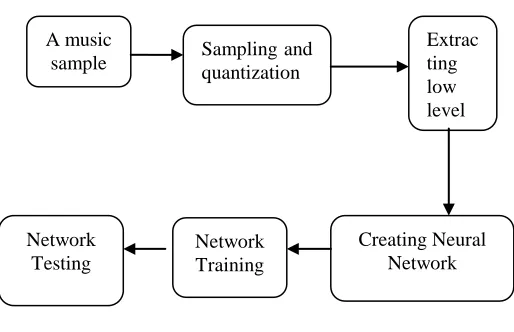
The overall schematic diagram in order to classify the

mood of the songs is shown in figure 1. The input to the

system is a song in wav form, while the output is a mood of

the defined types. The following figure reflects the

ISSN 2348 – 7968

Figure 1

We have taken the song as input and using Matlab’s

wavread function we sampled the audio WAV file and convert it into text format. These functions sample

the audio signal at 44.1 KHz and stored in the text

files. Sampling is a process of converting continuous

time domain signal into discrete signal. It can be done

in matlab using “wavread” function. wavread supports multichannel data, with up to 32 bits per

sample, and supports reading 24- and 32-bit .wav files.

We then extracted the audio based features: entropy of

the signal, energy of the signal, zero crossing rate,

spectral rolloff, spectral centroid, spectral flux, RMS

of the signal, and MFCC form the sampled file. A feed

forward neural network is created in this step. The

network is formed by selecting the best set of network

attributes. Two hidden layers are taken each layer

contains 10 neurons and default activation functions

are used for each layer. The network is trained with

the features matrix of 90 songs of three different

moods. Number of epochs is selected to 1000, training

goal is set to 0.1, learning rate is set to 0.05, training

time to 32, mem_reduc is set to 2 etc. After successful

training the network is then tested to the known moods

songs. Basically network is tested to draw out the

efficiency rate. Testing ensures implementation of the

system.

The network efficiency can be improved by applying

certain techniques that are based on the concept of

probabilistic reasoning. Baye’s Theorem is one such

concept. If one found satisfying results after applying

Baye’s reasoning it can then be implemented to increase

the efficiency rate but again remember it is purely based on

probabilistic reasoning, thus there are issues in adopting

this concept.

Bayes' Theorem is a theorem of probability theory

originally stated by the Reverend Thomas Bayes. It can be

seen as a way of understanding how the probability that a

theory is true is affected by a new piece of evidence. It has

been used in a wide variety of contexts, ranging from

marine biology to the development of "Bayesian" spam

blockers for email systems. In the philosophy of science, it

has been used to try to clarify the relationship between

theory and evidence. Many insights in the philosophy of

science involving confirmation, falsification, the relation

between science and pseudoscience, and other topics can

be made more precise, and sometimes extended or

corrected, by using Bayes' Theorem. These pages will

introduce the theorem and its use in the philosophy of

science.

Begin by having a look at the theorem, displayed

below. Then we'll look at the notation and

terminology involved.

P(A/B)= (P(A) * P(B/A)) / P(B)

Where,

P(A) and P(B) are probability of two events A

and B.

A music

sample Sampling and _quantization

Creating Neural Network Network

Testing

Extrac ting low level

ISSN 2348 – 7968

P(A/B) signifies probability of event A if event

B is true.

P(B/A) signifies probability of event B if event

A is true.

3.1 Features Extraction for Music

Classification

Feature extraction requires an in-depth understanding of

the signal processing theories. In this chapter we will be

discussing the theoretical aspects of these features and

feature extraction process.

1) Entropy: Entropy is a property that can be used to determine the energy not available for work. It is also a

measure of the tendency of a process. It is a measure of

disorder of a system.

Entropy refers to the relative degree of randomness. The

higher the entropy, the more frequently are signaling

errors. Entropy is directly proportional to the maximum

attainable data speed in bps. Entropy is directly

proportional to noise and bandwidth. It is inversely

proportional to compatibility.

Entropy also refers to disorder deliberately added to data

in certain encryption process.

2) Energy:

Signal energy refers to strength of

signal amplitude. In signal processing, the

energy

of a continuous-time signal x(t) is

defined as

Energy in this context is not, strictly speaking,

the same as the conventional notion of energy in

physics and the other sciences. The two concepts

are, however, closely related, and it is possible to

convert from one to the other:

where Z represents the magnitude, in appropriate units of measure, of the load driven by the signal.

For example, if x(t) represents the potential (in

volts) of an electrical signal propagating across a

transmission line, then Z would represent the

characteristic impedance (in ohms) of the

transmission line. The units of measure for the

signal energy

would appear as volt

2

-seconds,

which is not dimensionally correct for energy in

the sense of the physical sciences. After dividing

by

Z, however, the dimensions of E would

become volt

2

-seconds per ohm, which is

equivalent to joules, the SI unit for energy as

defined in the physical sciences.

3) Zero Crossing Rate:

It refers to number of

times the signal crosses zero line. The

zero-crossing rate

is the rate of sign-changes along a

signal, i.e., the rate at which the signal changes

from positive to negative or back. This feature

ISSN 2348 – 7968

and music information retrieval, being a key

feature to classify percussive sounds

[2]

.

ZCR is defined formally as

where is a signal of length and the indicator

function

is 1 if its argument is true and

0 otherwise.

In some cases only the "positive-going" or

"negative-going" crossings are counted, rather

than all the crossings - since, logically, between

a pair of adjacent positive zero-crossings there

must be one and only one negative zero-crossing.

For monophonic tonal signals, the zero-crossing

rate can be used as a primitive pitch detection

algorithm

4) Spectral Rolloff: Flatness of sound. The decrease in energy with increase in frequency, ideally described in the

sound source as 12 dB per octave. Spectral rolloff is

defined as the frequency where 85% of the energy in the

spectrum is below this point. It is often used as an indicator

of the skew of the frequencies present in a window.

5) Spectral Flux: It determines changes of spectral energy (variation of harmonics). A feature extractor that extracts

the Spectral Flux from a window of samples and the

proceeding window. This is a good measure of the amount

of spectral change of a signal.

Spectral flux is calculated by first calculating the

difference between the current value of each magnitude

spectrum bin in the current window from the

corresponding value of the magnitude spectrum of the

previous window. Each of these differences is then

squared, and the result is the sum of the squares.

6) Spectral Centroid: Spectral Centroid is the balancing point of sub-band energy distribution. It determines the

frequency area around which most of the signal energy

concentrates and is thus closely related to the time domain

ZCR feature.

It is also frequently used as approximation for a perceptual

brightness measure. A feature extractor that extracts the

Spectral Centroid. This is a measure of the "centre of

mass" of the power spectrum.

This is calculated by calculating the mean bin of the power

spectrum. The result returned is a number from 0 to 1 that

represents at what fraction of the total number of bins this

central frequency is.

7) Root Mean Square: It refers to the mathematical implementation of root of mean of square of the signal

value (discrete sampled value). A feature extractor that

extracts the Root Mean Square (RMS) from a set of

samples. This is a good measure of the power of a signal.

RMS is calculated by summing the squares of each sample,

dividing this by the number of samples in the window, and

finding the square root of the result.

8

) MFCC (Mel Frequency Cepstral Coefficient): Mel-frequency cepstral coefficients (MFCCs) are coefficients

ISSN 2348 – 7968

a linear cosine transform of a log power

spectrum on a nonlinear mel scale of frequency.

They are derived from a type of cepstral

representation of the audio clip (a nonlinear

"spectrum-of-a-spectrum"). The difference

between the cepstrum and the mel-frequency

cepstrum is that in the MFC, the frequency bands

are equally spaced on the mel scale, which

approximates the human auditory system's

response more closely than the linearly-spaced

frequency bands used in the normal cepstrum.

This frequency warping can allow for better

representation of sound, for example, in audio

compression.

MFCCs are commonly derived as follows:

1. Take the Fourier transform of (a windowed

excerpt of) a signal.

2. Map the powers of the spectrum obtained above

onto the mel scale, using triangular overlapping

windows.

3. Take the logs of the powers at each of the mel

frequencies.

4. Take the discrete cosine transform of the list of

mel log powers, as if it were a signal.

5. The MFCCs are the amplitudes of the resulting

spectrum.

3.2

Learning and Classification using

Neural Network

Learning using neural network requires input feature

matrix and output target matrix. The input feature matrix is

created from discrete samples values of the input songs for

training by calculating different audio features values.

We have taken the song as input and using Matlab’s

wavread function we sampled the audio WAV file and convert it into text format. These functions sample the

audio signal at 44.1 Khz and stored in the text files. We

then extract the audio based features entropy of the signal,

energy of the signal, zero crossing rate, spectral rolloff,

spectral centroid, spectral flux, RMS of the signal, and

MFCC form the sampled file.

We then supply the extracted audio features and their

expected outcomes as inputs to create the network. The

classifier is implemented using MATLAB’s Neural

Networking toolbox. The classifier is a feed forward neural

network with back propagation learning algorithm. Once

the classifier is trained we simulate the classifier and get

the mood of the song.

Process of creating Feedforward Neural Network:

Collect data: We have taken 90 songs (30 for each category : happy, sad and angry). We have extracted

10 lakhs discrete samples from the middle part of

song’s signal to reduce the length of each song. Then

we have calculated the values of seven features

described above using matlab script. We have

prepared feature input matrix of each song which will

be given as input to a feed forward neural network.

ISSN 2348 – 7968

each and 1 output layer with 3 neurons.The transfer

function of 2 hidden layers is “tansig” and “purelin”

respectively and the transfer function of the output

layer is “logsig”.

Configure the network :

In this process we can change the attribute values of

network to make the network learn in an efficient way.

Matlab code of configuring a network-

net.trainParam.epochs=1000;

net.trainParam.goal=.1;

net.trainParam.lr=0.05;

net.trainParam.time=32;

net.trainParam.mem_reduc=2;

where,

epochs signifies number of iterations of network.

goal signifies tolerance range under which output can vary.

lr is learning rate, which is one of the parameters which governs how fast a neural network learns and how effective

the training is.

Time signifies time taken by neural network to learn.

Mem_reduc is an attribute which signifies reducing the memory to increase efficiency.

Initialize the weights and biases :

The

configure

command configures the network object

and also initializes the weights and biases of the network;

therefore the network is ready for training. There are times

when you might want to reinitialize the weights, or to

perform a custom initialization. Initializing Weights (init)

explains the details of the initialization process. You can

also skip the configuration step and go directly to training

the network. The

train

command will automatically

configure the network and initialize the weights.

Weights are saved in network attributes “net.iw”.

Train the network:

Once the number of layers, and number of units in each

layer, has been selected, the network's weights and

thresholds must be set so as to minimize the prediction

error made by the network. This is the role of the training algorithms.

Train function is used to train the network.

Matlab code to train the network:-

net=train(net,p,t);

save 'network.mat''net';

Where

“net” is the network variable “p” is input feature matrix “t” is target matrix

Save function is used to save the network “net” in the file named ”network.mat”

Test the network:

Testing is done to check whether the network is producing

the desired output or not. We tested the network with 45

songs(15 for each category).

Use the network: If the testing is successful and the efficiency of results is around 60-70% then we can use

the network to test the new songs of unknown mood

by simulating the saved trained network.

4.0 Implementations, Results and

ISSN 2348 – 7968

We have implemented this system on windows

platform in MATLAB 7.0.1. Both GUI and the

classifier is implemented using MATLAB. Initially we

have collected the database of various Hollywood

songs in WAV format. We have taken songs from all

three moods. Out of all songs we have reserved 90

songs for training purpose, 30 songs from each of the

three mood i.e. happy, angry and sad. Songs are then

sampled and samples are then cut to fixed lengths i.e.

10 lakhs samples from middle of each song. The 8

selected audio features are then extracted from each

song and features values of all 90 songs are stored in a

feature matrix. This feature matrix is used as input

feature matrix with 8 rows containing features values

and 90 columns for 90 songs, for training the neural

network. Each column of this matrix represents

features of one song. An output target matrix is

constructed according to the input matrix representing

the known mood of the 90 songs. The output target

matrix contains 3 rows representing mood and 90

columns for 90 songs.

Neural Network can be created using “newff” function

in Matlab. NEWFF Creates a feed-forward back

propagation network. Since there are 8 input features,

initially we started with 6 hidden neurons. We ran the

training and testing sets through the network 10 times.

But there was always the requirement to have right set

of attribute values and the result of the simulation of

the network is not good as expected. Therefore we

then have chosen 2 hidden layers each layer

containing 10 neurons. The no. of iterations (epoch) is

most important. We kept the no. of epochs to 1000.

Though maximum amount of learning is done by 2000

epochs but it is by 1000 that the learning curve

becomes nearly horizontal. The performance function

value (goal) is kept to .01 during the training process.

Values around .002-.003 are the minimum

performance function values that we reach during the

training and the networks trained up to these values

produced satisfactory results .So we keep the value to

.01 because by that value the network would really be

trained enough. Learning rate is kept to .05. The no. of

epochs after which the status of the level of training

done is displayed (show) is kept to 50. Other

parameters are kept to default value. This time

network is trained 10 times to obtain the network that

can be efficiently adopted after adjusting some

network parameters. Then after training with 10

hidden neurons and fixed set of network attribute

values we have computed the results. In order to

increase the efficiency rate we have applied

probabilistic reasoning through “Bayes theorem”.

4.1 Performance Evaluation

Performance evaluation can be done by testing the

network with different songs with known mood and

check their efficiency rate.

With the 8 important features selected, the approach

was to determine how well the multilayer feed forward

neural network would classify the songs. First, we

determined how many hidden neurons should be in the

hidden layer of the network.

We have extracted a clip from a song (between 30-50

secs) and started the training. When we have tested

these results we didn’t get the desired efficiency so we

have decided to have a different approach. After

testing the new results obtained we have noticed that

ISSN 2348 – 7968

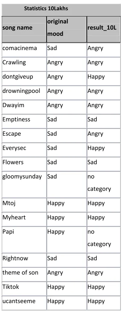
shows the results of this new testing scheme, a

comparison is shown between tested results through

the system and the original known mood the songs:

Statistics 10Lakhs

song name

original

mood

result_10L

Activate

Angry

Angry

Addicted

Sad

Angry

Ajks

Angry

Sad

Alldcold

Sad

Sad

Amyrica

Angry

Sad

Backst

Sad

Angry

beastie boys

Angry

Happy

Beforewebegu

n

Sad

Happy

Blameit

Sad

Sad

Bottomsup

Angry

Angry

Breakstuff

Angry

Happy

Breathme

Sad

Sad

Brick

Sad

Sad

Burndown

Angry

no

category

burnground

Angry

Angry

Camarada

Happy

Happy

Careless

Happy

Happy

chickenwire

Sad

Sad

claymoreparty

Angry

Sad

Statistics 10Lakhs

song name

original

mood

result_10L

comacinema

Sad

Angry

Crawling

Angry

Angry

dontgiveup

Angry

Happy

drowningpool

Angry

Angry

Dwayim

Angry

Angry

Emptiness

Sad

Sad

Escape

Sad

Angry

Everysec

Sad

Happy

Flowers

Sad

Sad

gloomysunday

Sad

no

category

Mtoj

Happy

Happy

Myheart

Happy

Happy

Papi

Happy

no

category

Rightnow

Sad

Sad

theme of son

Angry

Angry

Tiktok

Happy

Happy

ucantseeme

Happy

Happy

Table -1

We can see here in this testing we got 18 out 36 songs

are correctly matched. These 10 lakhs samples were

from the start of the song that does not ensure

ISSN 2348 – 7968

zeros in the starting duration which would not be

efficient.

Therefore we have decided to have another approach

and extracted samples from middle part of the song.

We have taken 10 lakhs fixed length samples from the

middle part of every song and then repeated the

process. Since there are 8 input features, initially we

started with 6 hidden neurons. We ran the training and

testing sets through the network 10 times. But there

was always the requirement to have right set of

attribute values. This time network is trained 10 times

to obtain the network that can be efficiently adopted

after adjusting some network parameters. This time we

then have chosen 2 hidden layers each layer

containing 10 neurons. The network goal, learning rate

and training time is adjusted such that to have the best

network that could be selected after modifying the

parameters values and testing some songs hand in

hand. Then after training with 10 hidden neurons and

fixed set of network attribute values we have

computed the results. In order to increase the

efficiency rate we have applied probabilistic reasoning

through “Baye’s theorem”.

Method of increasing efficiency:

P(A) is maximum component of any of the mood.

P(B) refers to the case when a song does not belong

to any of the category and the output matrix is

[0;0;0] (zero matrix).

P(B/A) refers to the probability of output matrix is

zero matrix when the maximum component refers to

original mood of the song.

Thus, the probability of maximum component refers

to the original mood when the output matrix is zero

matrix.

In our case,

P(A)=24/42;

P(B)=6/42;

P(B/A)=3/24;

P(A/B)=((24/42)*(3/24))/(6/42);

=1/2 = 50%

Baye’s Theorem gives satisfying results, thus we’ve

decided to implement Baye’s Theorem to increase

our efficiency rate. Statistics obtained after applying

Baye’s Theorem are is shown in Table-2

Test Statistics Table

Song name

original

mood

tested result

Activate

Angry

Angry

Addicted

sad

Angry

Ajks

angry

Angry

all d cold

sad

angry

Amyrica

angry

Angry

Backst

sad

Happy

beastie boys

angry

Angry

before we

begun

ISSN 2348 – 7968 Test Statistics Table

Song name

original

mood

tested result

blame it

sad

Happy

bottoms up

angry

no category

break stuff

angry

Happy

breathe me

sad

Sad

Brick

sad

Sad

burn down

angry

Angry

burn ground

angry

Angry

Camarada

happy

Sad

Careless

happy

Angry

chicken wire

sad

Sad

clay more

party

angry

Sad

coma cinema

sad

Happy

Crawling

angry

Angry

dont give up

angry

Angry

drowning

pool

angry

Happy

Emptiness

Sad

Sad

Escape

Sad

Angry

every second

Sad

Sad

Flowers

Sad

Sad

gloomy

Sunday

Sad

Sad

heal the

world

Happy

Sad

Test Statistics Table

Song name

original

mood

tested result

Mtoj

Happy

Sad

my heart

Happy

Happy

null sleep

Happy

Happy

Papi

Happy

Angry

right now

Sad

Angry

stuck in

infinity

Sad

Sad

the guest

Sad

Sad

the way We

am

Angry

no category

theme of son

Angry

Angry

Tiktok

Happy

happy and

angry

United

Happy

no category

waving flag

Happy

Happy

you cant see

me

Happy

Happy

Table- 2

We got 25 songs out of 42 test songs correctly

matched to the original mood. So our efficiency rate is

59.53% (around 60%).

ISSN 2348 – 7968

In this work we have characterized song into different

moods using multi layer feed forward neural network with

supervised back propagation learning algorithm. We have

taken 8 audio features to form one single feature vector

and then trained the network with audio features.

Training a neural network is a typical process. A network

must be trained with accurate set of feature values and with

accurate set of network attribute values. Features

extraction is the core part of determination of the mood of

a song that is highly dependent on features values. A

thorough, deep and accurate study must be made in order

to identify best set of features that can be extracted out of

an audio song. Any miss of accuracy will definitely

produce false results.

Experimental results show the robustness of the system.

The system classifies audio into happy, angry and sad

mood.

Although we’ve taken care of accuracy as best we can do,

still trained network has produced only 60% efficiency.

The mood classification system was developed as a

feasibility study for the development

of a system that would classify, successfully, music files

according to their mood . This section will discuss future

work that needs to be done in order to further study this

problem and develop such a system.

Biblography

[1] P. Ekman. An argument for basic emotions. Cognition

& Emotion, 6(3/4):169–200, 1992.

[2] J. A. Russell. Affective space is bipolar. Journal of

Personality and Social Psychology,37(3):345–356, 1979.

[3] J. A. Russell. A circumplex model of affect. Journal of

Personality and Social Psychology,39(6):1161–1178,

1980.

[4] R. E. Thayer. The Biopsychology of Mood and

Arousal. Oxford University Press, Oxford, 1989.

[5] R. E. Thayer. The origin of everyday moods: managing

energy, tension, and stress. Oxford University Press, New

York, 1996.

[6] A. Mehrabian. Pleasure-arousal-dominance: A general

framework for describing and measuring individual.

Current Psychology, 14(4):261–292, 1996.

[7] Y. Feng, Y. Zhuang, and Y. Pan. Music information

retrieval by detecting mood via computational media

aesthetics. In Proceedings of the IEEE/WIC International

Conference on Web Intelligence, page 235, Washington,

USA, 2003.

[8] [24] P.N.Juslin. Cue utilization in communication of

emotion in music performance: relating performance to

perception.Journal of Experimental Psychology: Human

Perception and Performance, 26(6):1797–1813, 2000.

[9] S. Dixon. A lightweight multi-agent musical beat

tracking system. In Proceedings of the Pacific Rim

ISSN 2348 – 7968

[10] K. Hevner. Experimental studies of the elements of

expression in music. The American Journal of Psychology,

48(2):246–268, 1936.

[11] C.H. Chen, M.F. Weng, S.K. Jeng, and Y.Y.

Chuang.Emotion-Based Music Visualization Using

Photos.LNCS, 4903:358–368, 2008.

[12] P. R. Farnsworth. A study of the hevner adjective list.

The Journal of Aesthetics and Art Criticism, 13(1):97–103,

1954.

[13] M. G. Rigg. What Features of a Musical Phrase Have

Emotional Suggestiveness?,volume36 of Bulletin of the

Oklahoma Agricultural and Mechanical College.

Oklahoma Agricultural and Mechanical College,

Stillwater, Oklahoma, 1939.

[14] M. G. Rigg. The mood effects of music: A

comparison of data from four investigators.The Journal of

Psychology, 58:427–438, 1964.

[15] K. B. Watson. The nature and measurement of

musical meanings. In Psychological Monographs, volume

54, pages 1–43. The American Psychological Association,

Evanston, IL, 1942.

[16] L. Lu, D. Liu, and H.J. Zhang. Automatic mood

detection and tracking of music audio signals. IEEE Trans.

Audio, Speech & Language Process, 14(1), 2006.

[17] T.L. Wu and S.K. Jeng. Probabilistic estimation of a

novel music emotion model. In 14th International

Multimedia Modeling Conference. Springer, 2008.

[18] S. Kim, S. Kim, S. Kwon, and H. Kim. A music

summarization scheme using tempo racking and two stage

clustering. IEEE Workshop on Multimedia Signal

Processing, pages 225–28,2006.

[19] L. Lu, D. Liu, and H.J. Zhang. Automatic mood

detection and tracking of music audio signals. IEEE Trans.

Audio, Speech & Language Process, 14(1), 2006.

[20] C.C. Liu, Y.H. Yang, P.H. Wu, and H.H.

Chen.Detecting and classifying emotion in popular music.

In JCIS, 2006.

[21] Sanjay Jain and R.S. Jadon, “Audio Based Movies

Characterization using Neural Network”, published in

International Journal of Computer Science and

Applications(IJCSA ISSN 0974-1003), Vol 1 No.2, PP 87-

91, Aug, 2008.

[22] Sanjay Jain and R.S. Jadon, “Features Extraction for

Movie Genres Characterization”, in Proceeding of

WCVGIP-06, 2006.

[23] T. Li and M. Ogihara. Content-based music similarity

search and emotion detection.In Proceedings of the IEEE

International Conference on Acoustics, Speech, and Signal

Processing, volume 5, pages 705–708, 2004.

[24] G. Tzanetakis and P. Cook. Marsyas: a framework for

audio analysis. Organised Sound, 4(3):169–175, 1999.

[25] A. Tellegen, D.Watson, and L. A. Clark. On the

dimensional and hierarchical structure of affect.

Psychological Science, 10(4):297–303, 1999.

[26] D.YangandW.Lee. Disambiguating music emotion

ISSN 2348 – 7968

International Conference on Music Information Retrieval,

Barcelona,Spain, 2004.

[27] M. Tolos, R. Tato, and T. Kemp. Mood-based

navigation through large collections of musical data. In

Consumer Communications and Networking Conference,

pages 71–75,Las Vegas, USA, 2005.

[28] A. Wieczorkowska, P. Synak, R. Lewis, and Z. Ras.

Extracting emotions from music data. In Proceedings of

the 15th International Symposium on Methodologies for

Intelligent Systems, Saratoga Springs, USA, 2005.

[29] ww.mathworks.com/help/pdf_doc/nnet/nnet_ug.pdf.