Comparison of two methods of mathematical modeling in hydrodynamic sealing gap

(1)

a

Corresponding author: jkrutil@seznam.cz

Comparison of two methods of mathematical modeling in hydrodynamic

sealing gap

Jaroslav Krutil1,a, Kamil Fojtášek2, Lukáš Dvoák 3

1

Brno University of Technology, Faculty of Mechanical Engineering, Victor Kaplan Dept. of Fluid Engineering, Technická 2896/2, Brno 61669, Czech Republic

2, 3

VŠB-Technical University of Ostrava, Faculty of Mechanical Engineering, Department of Hydrodynamics and Hydraulic Equipment, 17. listopadu 15/2172, Ostrava 70833, Czech Republic

Abstract.The aim of work is to compare two possible methods of mathematical modeling of hydrodynamic instabilities. This comparison is performed by monitoring the formation and evolution of Taylor vortices in hydrodynamic sealing gap. Sealing gaps are a part of the hydraulic machines with the impeller, such as turbines and pumps, and they have an effect on the volumetric efficiency of these devices. This work presents two examples of sealing gaps. These examples are closed sealing gap and modified sealing gap with expansion chamber. On these two examples are applied procedures of solution contained in CFD software (ANSYS Fluent 14.5). In ANSYS Fluent is two possible basic approaches of solution this task: the moving wall method and the sliding mesh method. The result of work is monitoring the impact of the expansion chamber on the formation of hydrodynamic instabilities in the sealing gap. Another result is comparison of two used methods of mathematical modeling, which shows that both methods can be used for similar tasks.

1 Introduction

Hydrodynamic sealing gaps are an integral part of hydraulic machines with impellers. Basically it is a narrow gap which is disposed between the rotor and the stator of the hydrodynamic machine.

Sealing gap acts as a bearing element, which prevents mutual contact between the rotor and stator. This sealing gap combines the function of damper, spring and mass elements. However, this applies only if it is properly designed. If this element is improperly designed, it can cause unwanted self-excited vibrations of the rotor. It may also cause the flow field destabilization from which subsequently follows the vibrations and loudness of the machine. In extreme cases, it can lead to failure of the hydrodynamic machine.

For these reasons, from the industrial and professional experiences point of view it is very important to explore the events that are associated with the function and behavior of sealing gaps. The interaction of the rotor of the pump with liquid causes forces that fundamentally affect the dynamics of the rotor [1, 2]. These forces are dependent on the pressure gradient, speed, acceleration and deflection of the rotor, the density and viscosity of the liquid. One of the many tools that can well describe the processes taking place inside the sealing gap is Computational Fluid Dynamics (CFD) simulation. This allows the simulation of the behavior inside the sealing

gaps under different working conditions. The solution is based on the method of control volumes. The used tool for the solution is numerical program ANSYS Fluent 14.5. The most important process that can occur is the instability of the Couette flow. As a result of this instability is the creation of Taylor vortices. These Taylor vortices are formed between two concentric cylinders. The inner cylinder is rotated at a certain speed. On reaching the critical speed of rotation there are formed axially symmetric toroidial vortex structures - Taylor vortices [3].

The aim is to show the advantages and disadvantages of two possible methods of mathematical modeling of hydrodynamic instabilities which are arising in sealing gaps. There are used two approaches in CFD solution. The method using the moving wall and the method using the sliding mesh. The comparison of both used methods can provide us information that will facilitate subsequent mathematical modeling of similar problems.

Mathematical models were created for two types of sealing gaps. The sealing gap with classic shape and modified sealing gap with the expansion chamber. The expansion chamber reduces flow losses and increases the flow efficiency and thus the overall efficiency of the machine.

C

Owned by the authors, published by EDP Sciences, 2015

(2)

2 Theory

If the real fluid flow between two concentric and moving cylinders there are formed the hydrodynamic instabilities. Taylor-Couette flow is a classic case of a conditional unstable flow that occur under certain conditions. Taylor's critical number is a criterion for the assessment of the stability of the flow. The various flow regimes were defined by experiments [4]. The criterion for transfer of the individual states there is a dimensionless Taylor number that can be expressed as [5, 6]:

ܶ ൌȳ ή ݎ_߭ଵή ݀ή ඨ_ݎ݀

ଵ൒ ܶ஼ଵ ൌ ͶͳǤ͵Ǥ

(1)

Definition of the Taylor number is more, such as

ܶଶ_ൌͶ ή ݀ଶή ȳଶ

߭ଶ ή

ߟଶ

ߟଶ_{െ ͳ}ǡ (2)

where

ߟ ൌଵ

ଶǤ (3)

In general, the most authors divides Taylor-Couette flow to these modes [4, 7]:

• Taylor vortex flow

The creation of the periodic instabilities in the form of annular axisymmetric Taylor vortices with a stable character is described by the critical value of ܶ_௖ଵ. If the condition ܶ ൐ ܶ_௖ଵ൒ ͶͳǤ͵ is true, then leads to the creation of this instability.

• Wave vortex flow

This flow is beginning to appear after a further increase in speed of internal cylinder (and also increase of the value of T). When ܶ_௖ଶ൐ ܶ_௖ଵ there is a wave-motion of vortices in the circumferential direction. Critical number ܶ_௖ଶ is dependent on the geometry of the gap and properties of the liquid, and there is approximately in the range ܶ_௖ଶൎ ሺͳǤͳ െ ͳͲͲሻ ή ܶ_௖ଵ.

• Modulated wave vortex flow

In this mode, appears the modulation wave-motion of vortices. There is a frequency of azimuthal waves which modulates vortices and does not depend on the frequency of wave motion. Gradually leads to the narrowing and expansion of corrugated toroidal vortices in the circumferential direction. The number of waves is in the range 3 - 7.

• Chaos

Chaotic mode is in the range ܶ_௖ଶ ൎ ሺͳͲͲ െ ͳͲͲͲሻ ή ܶ௖. It is highly dependent on the ratio of radii

ߟ. Further increase of number ܶ is leading to the turbulent effects, which disrupting vortices.

These modes of flow correspond only the case when the outer cylinder is stationary.

3 Mathematical modeling

3.1 Governing equation

The basic equations that describe the flow of real liquids in a given volume or in the given environment are [4, 8]: • The law of conservation of mass (continuity equation)

The equation of continuity describes the law of conservation of mass, ie the relationship between the incoming and outgoing mass in a given volume.

߲ݑ௝

߲ݔ௝ ൌ ͲǤ (4)

• The law of conservation of momentum (Newton's second law)

The balance of forces in the flow of real liquid is given by Navier-Stokes equations, which express the relationship between the inertia force and external force. The external force is equal to the sum of the mass force and surface forces (pressure and friction).

߲ݑ௜ ߲ݐ ൅ ߲൫ݑ௜ݑ௝൯ ߲ݔ௝ ൌ െ ͳ ߩ ߲݌ ߲ݔ௜൅ ߭ ߲ଶ_ݑ ௜ ߲ݔ௝ଶ ൅ ݂௜Ǥ (5)

In general form these equations are system of partial differential equations and there are suitable for laminar or turbulent flow. They can be solved by the following methods: differential method, finite volume method, finite element method and spectral method. In modeling of flow is used finite volume method, which consists of three basic points [9]:

- dividing the area into discrete volumes using by curvilinear grid,

- balancing the unknown quantities in individual finite volume and discretization,

- numerical solution of the discretized equations in general form.

3.2 Numerical procedure – Approaches solutions in the CFD

This work describes two basic approaches to solutions. The first variant solves the movement of the inner cylinder using by the moving wall method. The second variant solves this movement using by sliding mesh method. Both of these variations have their advantages and disadvantages and possibilities of use. More information on moving wall and sliding mesh (functions with this name in ANSYS Fluent software) are listed in [10]:

1) Moving wall variant A

In the tab Walls is necessary to check the item moving wall, which allows you to define any wall motion (translational and rotational motion). After this step, it is possible to define a user-desired rotation speed [11].

2) Sliding mesh variant B

(3)

different zones are connected to each other with not-conformal interface. These types of tasks are solved especially as a time dependent. At each time step occurs to update interfaces and reflect the new position of cells in each zone. Another important characteristic is that the motion of the nodes must be such, that two neighboring interfaces remain permanently in contact each other. Through this interface can lead to the free flow of fluid from one zone to another (in both directions) [11]. The sliding mesh is shown in Figure 1.

Figure 1. Layout of boundary conditions for sliding mesh

3.3 Numerical solution of practical problems – sealing gap closed

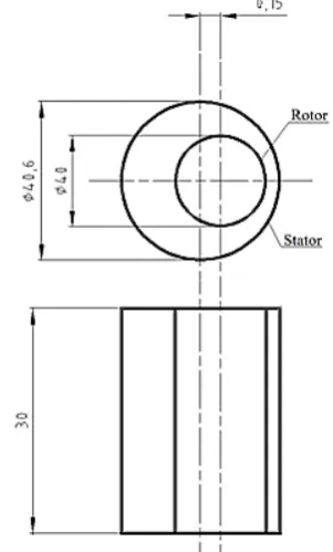
In this part the focus is on solving the real task of sealing gap by using the numerical CFD program ANSYS Fluent. Dimensions of solved task are based on the real device (SIGMA Lutín). For this device took place series of test experiments carried out in the workplace Department of Fluid Engineering V. Kaplan, Brno University of Technology. Description and course of physical experiments are in research reports [12-14]. Simplification of the device lies in the complete closure of the inlet and outlet chambers (input and output annulus). The shape and dimensions of sealing gap are shown in the Figure 2.

Since there are two ways of solving the problem of similar tasks, it is necessary for each of these methods create a special geometry. Detailed shape of the geometry with description of zones is evident from Figure 3a and 3b. The fundamental difference in geometry creation is mainly in the number of zones that contain individual variants. While the A variant (variant using moving wall) is needed only one zone (the movement is defined directly on the wall of the rotor). For variant B (using a sliding mesh) requires two zones. Rotational movement is defined at a very small layer of liquid which is rotated by the same speed as the rotor. And that leads to sliding upon mutual non-conformal interface.

The boundary conditions Figure 4 are defined for all walls as a Wall. In the variant A was the wall of the rotor defined as moving wall. In variant B the wall of the rotor was defined as a stationary wall (movement is performed using a sliding mesh). The diversity in the solutions of both variants leads to differences between computational grids that cover the solved area. Comparison between the

two variants of grid is detailed shown in Figure 5a and Figure 5b.

Figure 2. Schematic representation of the solved area

Figure 3a. Variant A (using moving wall)

Figure 3b. Variant B (using sliding mesh)

The theory shows that the angular velocity has a significant influence on the formation of Taylor vortices. It was selected the following list of angular speed Table 1 (critical Reynolds number for small eccentric gap is ܴ݁௖௥௜௧ ൌ ͳͲͲͲ) [4, 5].

Zone II

Zone I

(4)

Figure 4. Geometry with boundary conditions

Figure 5a. Variant A – detailed grid

Figure 5b. Variant B – detailed grid

From the calculations is evident that the variants with ͳǤʹͷ and ͳͲݎ݁ݒݏିଵare responsible to laminar flow and variant with ͷͲݎ݁ݒݏିଵ corresponds to turbulent flow. It is also considered when choosing the viscous mathematical model in ANSYS Fluent. After a several test calculations it has been found that the instability can be visualized only by using a laminar model. All turbulent models failed to show any swirl and the Taylor vortices does not arise. Which is the first important findings that were identified. Theoretical calculations of Taylor number Table 1 show that the formation of Taylor vortices is expected for tasks with speed ͳͲ and ͷͲݎ݁ݒݏିଵ_.

Table 1. List of compared variants

Revolutions Angular

velocity

Reynolds number

Taylor number

݊[rev s-1] ߗ [rad s-1] ܴ݁ [-] ܶ_௖ [-]

1.25 7.8539 70.6851 10.6027

10 62,8319 565.4871 84.8231

50 314,1593 2827.4337 424.1151

Recrit = 1000 Tcrit = 41.3

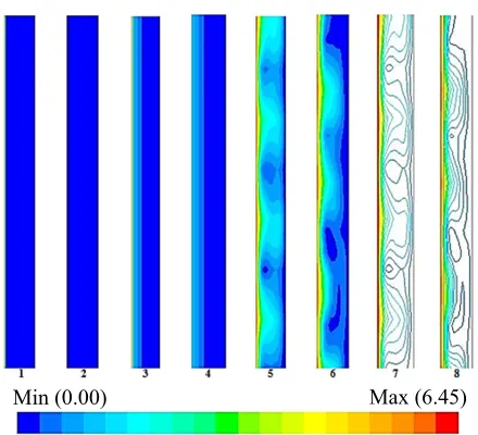
The main criterion for the assessment of formation hydrodynamic instabilities is the velocity field. With suitably placed cuts (across the widest part of annular) are evaluated contours of velocity. Figure 6 shows the contours of velocity, which suggests the possible formation and evolution of toroidal vortex structures for each variant. Descriptions of variants which corresponding with a Figure 6 are indicated in Table 2:

Table 2. Description of the variant in Fig.6

Revolutions

n [rev s-1] Used method Evaluation

1 1.25 Moving wall Filled contours 2 1.25 Sliding mesh Filled contours 3 10 Moving wall Filled contours 4 10 Sliding mesh Filled contours 5 50 Moving wall Filled contours 6 50 Sliding mesh Filled contours 7 50 Moving wall Unfilled contours 8 50 Sliding mesh Unfilled contours

Figure 6 shows that the formation of Taylor vortices occurs only for variants with speeds reaching ݊ ൌ ͷͲݎ݁ݒݏିଵ_{. Perspicuous creation of these vortices can be} seen in both variant A and B. It is interesting that the according to theory Table 1, should be the creation of instability also in speed ݊ ൌ ͳͲݎ݁ݒݏିଵ. However, this has not been confirmed by numerical simulation. In variant 3 and 4 does not create a swirl but as compared to variant for ݊ ൌ ͳǤʹͷݎ݁ݒݏିଵ is evidently that the velocity field is starting to be significantly deformed and slightly unstable.

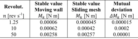
Another parameter that was monitored during numerical simulation is the torque moment of rotor. Comparison of results represents a Table 3, which is complemented by the deviation of both variants.

Table 3. Numerical evaluation of torque moment

Revolut. Stable value Stable value Mutual

deviation Moving wall Sliding mesh

݊ [rev s-1] ܯ_௞ [N m] ܯ_௞ [N m] ߂ܯ_௞ [N m]

1.25 0.00006 0.000045 0.000015

10 0.00062 0.00042 0.0002

50 0.00258 0.00257 0.00001

From the obtained results it is know that the differences between the moments of the variant A and variant B are almost negligible. We can say that the evaluation of the torque moment does not depend on the chosen variant.

The last significant variables that were recorded in the numerical simulation are the components of forces ݂ݔ and ݂ݕ depending on the time. In Figure 7 are shown components of forces for variant with moving wall and in Figure 8 are variant with sliding mesh. The difference between the both variants is especially in the course of Wall Stator

(5)

force. In the variant with using sliding mesh is a significant oscillation of each component of force. A variant with moving wall does not show this oscillation and have a significantly smoother course of force. In terms of numerical values of individual components, the results are almost identical in both variants. The numerical values for each force components are listed in Table 4. This table also includes the mutual deviation of forces. These differences are very slight. This fact again confirms the assumption that it is possible to use both variants for solve similar types of task. It is also evident that the all forces has been gradually almost stabilized.

Figure 6. Contours of the velocity field

Table 4. Numerical evaluation of force components

Revolutions Stable value – Moving wall Stable value – Sliding mesh Mutual deviation

݊ [rev s-1] ݂ [N] ݂ [N] ߂݂ [N]

݂ݔ ݂ݕ ݂ݔ ݂ݕ ݂ݔ ݂ݕ

1.25 0.00139 0.182 0.0022 0.181 0.00081 0.001

10 0.109 1.607 0.106 1.616 0.003 0,.009

50 6.332 11.458 4.684 10.445 1.648 1.013

Figure 7. The course of force components ݂ݔ and ݂ݕ – Variant A

Figure 8. The course of force components ݂ݔ and ݂ݕ – Variant B

Min (0.00) Max (6.45)

Time t (s) _Time_t_(s)

Force

f

x

(N

)

Force

fy

(N

)

Timet(s) Time t (s)

Force

f

x

(N

)

Force

fy

(N

(6)

3.4 Numerical solution of practical problems of sealing gap – modified task

Sealing gap is usually not fully closed (it has open input and output). This work is complemented by the task which has more realistic character. The original geometry is extended by chamber. This chamber change the character of the flow (pressure gradient) and in the modified task is set the pressure input and output. Both pressure conditions (pressure inlet and outlet) reach the same pressure ݌ ൌ ͲǤͳܯܲܽ. The pressure difference thus corresponds to the pressure gradient ߂݌ ൌ Ͳܯܲܽ. The shape of the chamber and their dimensions are shown in Figure 9 and Figure 10.

Figure 9. Modified model

Figure 10. Size of chamber

The mesh which is covered the body of sealing gap corresponds to the previous task, but is complemented by

a mesh of chamber. The cells in the chamber are compressed towards the body of the rotor. This compression of cells provides better convergence of task and we can achieve more accurate results of numerical simulations. In Figure 11 is detail of the chamber. From this figure it is obvious the layout of cells in the chamber and their shape. All other boundary conditions remain exactly the same as in the previous task.

Figure 11. The shape of mesh inside the chamber

The stable velocity field (at the speed of the rotor ݊ ൌ ͳǤʹͷݎ݁ݒݏିଵ_{) it starts to deformed into the transition} state (the rotation speed of the rotor ݊ ൌ ͳͲݎ݁ݒݏିଵ). A further increase in speed (݊ ൌ ͷͲݎ݁ݒݏିଵ) it is a phase where the laminar flow becomes to turbulent, and turbulence (chaos) arises. In Table 5 are indicated the description of variants which correspond with the Figure 12.

Table 5. Description of the variants in Fig.12

Revolutions

Used method Evaluation

n [rev s-1]

1 1.25 Moving wall Filled contours 2 1.25 Sliding mesh Filled contours 3 10 Moving wall Filled contours 4 10 Sliding mesh Filled contours 5 50 Moving wall Filled contours 6 50 Sliding mesh Filled contours 7 50 Moving wall Unfilled contours 8 50 Sliding mesh Unfilled contours

As in the previous task, the torque moment on the wall of rotor has been monitored. For both methods has been achieved approximately identical results (in steady state). Their mutual numerical comparison is in the Table 6. In this table are also calculated mutual deviations. It is evident that the results of this deviations in both variants are almost identical.

Table 6. Numerical evaluation of torque moment

Revolut. Stable value Stable value Mutual

deviation Moving wall Moving wall

݊ [rev s-1] ܯ_௞ [N m] ܯ_௞ [N m] ߂ܯ_௞ [N m]

1.25 0.000054 0.000053 0.000001

10 0.000494 0.000489 0.000005

50 0.003494 0.003212 0.000282

Pressure outlet

(7)

Finally, it was made a comparison of forces components ݂ݔ and ݂ݕ. It was monitored their total course depending on time. Figure 13 and 14 indicate how the forces behaved and evolved. From the mutual comparison of the two variants shows that the courses of both forces have almost identical character. Also the values of these forces are almost identical.

In variant A the course of forces are more smoother than variant B. In variant B there are considerable oscillations in the course of time. This effect can be most observed in the mutual comparison of forces ݂ݕ. Since there was no stabilization of forces (especially at high speeds ݊ ൌ ͷͲݎ݁ݒݏିଵ), this task does not contain a table of numerical evaluation.

Figure 12. Contours of the velocity field

Figure 13. The course of force components ݂ݔ and ݂ݕ – Variant A

Figure 14. The course of force components ݂ݔ and ݂ݕ– Variant B

Min (0.00) Min (6.45)

Force

f

x

(N

)

Force

fy

(N

)

Time t (s) Time t (s)

Time t (s)

Force

f

x

(N

)

Force

fy

(N

(8)

4 Conclusion

This work describes the modeling of rotary motion of cylinder by the finite element method, which is located concentrically with the second cylinder. There are two ways how solve this type of problems. The variant using the moving wall and variant using the sliding mesh. Under the certain conditions occur the unstable flow, which may lead as a result the formation of vortical structures also called Taylor vortices. Taylor-Couette instability may not lead directly to the formation of turbulent flow. May be changed only the character of the laminar flow. The fully developed turbulence is in the final stage when it is significantly exceeded the critical Taylor number. In the document are solved two task with specific boundary conditions that allow the formation of vortex instabilities. The results show, the both of these methods that have been used for mathematical modeling can be applied to this type of task. The comparison of both methods shows:

Method using moving wall:

൅ Fewer demands on mesh quality. ൅ Simple setting of calculation. ൅ Very good convergence.

െ Not possible to apply the method for a more complex tasks (combination of two or more movements).

Method using sliding mesh:

൅ The possibility to apply the method on more complex tasks (combination of two or more movements – for example the body makes rotational movement and additionally precessional movement).

൅ Good convergence.

െ High demands on mesh quality (especially in the total number around the circumference of the cylinder).

െ More complicated calculation settings. െ More complicated geometry creation. െ Longer calculation time.

െ Due to the interpolation of variables between the sliding mesh may occur less accurate calculation and may not Taylor vortices arise.

Acknowledgements

This work was supported by the project CZ.1.07/2.3.00/30.0005 of Brno University of Technology and by the project SP2015/95 of VŠB-TU Ostrava.

References

1- M.D. Sinnott, P.W. Cleary, Prog. in Comput. Fluid Dyn., Vol.10 (2010)

2- M. Kozdera, Jour. of App. Sci. in Thermodyn. and Fluid Mech., Vol.5, (2010)

3- R. Gupta, D.F. Fletcher, B.S. Haynes, Chem. Engi. Sci., Vol.64, (2009)

4- R.B. Bird, W.E. Stewart, N.N. Lightfoot, Transport Phenomena, (2002)

5- T.E. Faber, Fluid Dynamics for Physicists, (1995)

6- S. Dong, Jour. of Fluid Mech., Vol.587, (2007) 7- J. Farnik, Investigation of the instabilities in the gap

between two relative rotating concentrical cylinders, (2007)

8- F. Pochyly, S. Fialova, M. Kozubkova, M. Bojko, IOP Conf. Ser.: Earth Environ. Sci. 15,(2012)

9- M. Kozubkova, Modeling of fluid flow FLUENT CFX, (2008)

10-Ansys, Inc., ANSYS FLUENT 13.0 - Theory Guide (2011)

11-Ansys, Inc., ANSYS FLUENT 13.0 - User's Guide (2011)

12-V. Haban, M. Hudec, F. Pochyly, F. J. Archalous, N. Novakova, Experimental research on the effects of additional hydrodynamic fluid in the gaps I, (2012) 13-V. Haban, M. Hudec, F. Pochyly, N. Novaková, D.

Jasikova, M. Kotek, Experimental research on the effects of additional hydrodynamic fluid in the gaps II, (2013)

14-F. Pochyly, J. Krutil, Hydrodynamic effects of the sealing gap, (2013)