NONLINEAR SYSTEMS WITH MULTIPLICITY
Kerning Ma
UCL
A th e sis subm itted for the degree of Doctor of Philosophy of the
University of London
D epartm ent of Chem ical Engineering
University College London
London WCIE 7 JE
All rights reserved
INFORMATION TO ALL USERS
The quality of this reproduction is dependent upon the quality of the copy submitted. In the unlikely event that the author did not send a complete manuscript and there are missing pages, these will be noted. Also, if material had to be removed,
a note will indicate the deletion.
uest.
ProQuest 10016085
Published by ProQuest LLC(2016). Copyright of the Dissertation is held by the Author. All rights reserved.
This work is protected against unauthorized copying under Title 17, United States Code. Microform Edition © ProQuest LLC.
ProQuest LLC
789 East Eisenhower Parkway P.O. Box 1346
A b stra ct 5
D ed ica tio n 7
A ck n ow led gem en ts 8
1 In tro d u ctio n 9
1.1 General O v erv iew ... 9
1.2 O b je c tiv e s ... 14
1.3 Outline of the T h e s i s ... 14
2 L iterature R ev iew 16 2.1 Basic Concepts and Properties of Nonlinear Systems ... 17
2.1.1 F u n d a m e n ta ls... 17
2.1.2 Properties of S o lu tio n s ... 18
2.1.3 The Concept of Bifurcation A n a l y s i s ... 20
2.2 The Concept of Controllability in Process Engineering... 23
2.3 Limitations on C o n tro lla b ility ... 27
2.3.1 The Concept of Zeros and Zero D y n a m ic s ... 27
2.3.2 Perfect C o n t r o l ... 30
2.4.1 Input Multiplicity and RHP Z e ro s... 38
2.4.2 Control Problems Associated with Input Multiplicity . . . 40
2.5 An Overview of Controllability Analysis Techniques and Process Design Methods for Improved C o n tro llab ility ... 43
2.5.1 D efinitions... 43
2.5.2 Techniques for Controllability A n a ly s is ... 44
2.5.3 Design M ethods for Improved C ontrollability... 48
2.6 C o n c lu sio n s ... 53
3 A N e w A n a ly sis M eth o d ' 55 3.1 In tro d u c tio n ... 56
3.2 Bifurcation Analysis ... 57
3.3 Problem F o rm u la tio n ... 60
3.4 Solution M ethod ... 64
3.5 Illustration: van de Vusse Reactor Example ... 66
3.5.1 Analysis for the van de Vusse R e a c to r... 68
3.5.2 Comparison with Analytical Solutions ... 69
3.5.3 S u m m a r y ... 75
3.6 C o n c lu sio n s ... 75
4 P ro cess M od ification for Im proved C on trollab ility 76 4.1 In tro d u c tio n ... 77
4.2 Process Modification Methodology for Improved Static Controlla bility ... 77
4.2.1 Economically Optimal D e s i g n ... 78
4.2.2 Controllability Analysis for the “Base-Case” Design . . . . 79
4.3.1 Process D escrip tio n ... 83
4.3.2 Analysis for the Given P ro c e ss... 84
4.3.3 Process Design Modifications ... 88
4.3.4 Closed-Loop S im u la tio n s... 90
4.4 C o n c lu sio n s ... 95
5 C ase S tu d ies 96 5.1 Case Study I: A Reactor-Separator System w ith R e c y c l e ... 98
5.1.1 In tro d u c tio n ... 98
5.1.2 Process D escrip tio n ... 99
5.1.3 Process Model E q u a tio n s... 100
5.1.4 Controllable Analysis for the Base Case Design ... 105
5.1.5 Process Design Modifications ... 107
5.1.6 S im u la tio n s ...113
5.1.7 S u m m a r y ...118
5.2 Case Study II: An Industrial Polymerization R e a c t i o n ... 119
5.2.1 In tro d u c tio n ...119
5.2.2 Process Model and Optimal O peration D e s ig n ... 120
5.2.3 Analysis for the Base Case D e sig n ...123
5.2.4 Effects of Design and Operation P a r a m e t e r s ... 131
5.2.5 Process Design Modifications ... 138
5.2.6 Closed-Loop S im u latio n s... 140
6 C on clusion s and Future W ork 146
6.1 Summary of F in d in g s ... 146
6.1.1 New Method for Analysis ... 146
6.1.2 Process Design Modifications for Improved Controllability 148 6.2 Key Contributions ... 149
6.3 Recommendations for Further W o rk ... 150
A A cron ym s 153 B Zero D y n a m ics 155 B .l In tro d u c tio n ...155
B.2 M athematical P r e lim in a r ie s ... 156
B.2.1 Lie D e r iv a tiv e s ...156
B.2.2 Lie B ra c k e ts ... 156
B.3 Nonlinear Inversion: Zero D y n am ics... 157
B.3.1 Relative Order ...158
B.3.2 Normal F o rm s ...158
B.3.3 Nonlinear In v e rsio n ... 161
B.3.4 Zero D y n a m ic s ...162
C N u m erical T echniques in B ifu rcation P ro b lem s 165 C .l In tro d u c tio n ...165
C .2 Continuation of Solutions ... 166
C.2.1 Regular Solution P a t h s ...166
C.2.2 F o ld s ...167
C.2.3 Natural Param eter Continuation ... 168
C.2.4 Pseudo-arclength Continuation ... 169
C.3.2 Bifurcation T h e o r e m ...171
C.3.3 Detection of Bifurcation P o i n t s ...172
2.1 Summary of the typical controllability analysis measures in the
lite ra tu re ... 45
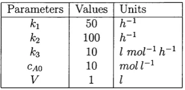
3.1 Param eters and values for van de Vusse r e a c t o r ... 68
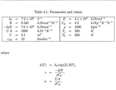
4.1 Param eters and v a l u e s ... 84
4.2 Process design modification results for the exothermic reaction . . 90
4.3 Param eters and operation values for the base-case and modified designs for the exothermic CSTR at steady s t a t e ... 90
5.1 Param eters and values for the optimal d esig n ... 105
5.2 Modification results of the reactor-separator system for cost weights: 7^ = l, Q = 5, and W = 10 112
5.3 Modification results of the reactor-separator system for cost weights: 7e = 0.15, Q = 0.55, and W = 1000 ... 113
5.4 Kinetic p a r a m e te r s ... 124
5.5 Process design and operation param eter v a lu e s ...124
1.1 Illustrative example: van de Vusse r e a c t o r ... 10
1.2 Steady-state solution relationship between input and output . . . 12
2.1 Two possible types of multiplicity, a) input multiplicity; b) output
multiplicity... 36
3.1 Schematic diagram of the van de Vusse r e a c to r... 66
3.2 Steady state solutions showing input multiplicity condition infor
mation for the van de Vusse reactor. Square: input multiplicity
co n d itio n ... 70
3.3 Steady state solutions showing input multiplicity condition with
variation of cao for van de Vusse reactor. Solid line: steady states
for a fixed cao ; dashed line: input multiplicity condition with
variation of c a o... 70
3.4 Locus of input multiplicity condition between inlet flow rate F and
feed composition c a o... 71
3.5 Contour of input multiplicity conditions as inlet flow rate, output,
and inlet concentration change for the van de Vusse reactor . . . . 71
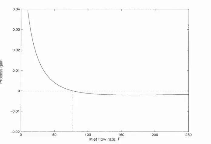
3.6 Process gain as a function of inlet flow rate for the van de Vusse
4.1 Steady-state solutions showing input multiplicity condition with
variations of inlet tem perature. Square: input multiplicity con
dition; dashed line: input multiplicity condition with variation of
inlet te m p e r a tu r e ... 86
4.2 Locus of inlet flow rate versus inlet tem perature at input multi
plicity c o n d itio n ... 86
4.3 Input multiplicity condition between the reactor tem perature, inlet
flow rate and inlet t e m p e r a t u r e ... 87
4.4 Input multiplicity condition between the inlet flow rate, inlet tem
perature, and reactor volum e... 87
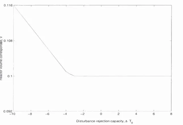
4.5 The relationship between design param eter and disturbance rejec
tion a b ility ... 91
4.6 Profiles of input and output for the initial design, V = 0.1 m^, for
disturbance rejection of inlet tem perature: —4 K and 92
4.7 Profiles of input and output for the initial design, V = 0.1 m^, for
rejection of —5 K change in the inlet te m p e r a t u r e ... 92
4.8 Profiles of input and output for the initial design, V = 0.1 m^, for
rejection of —4 K change in the inlet te m p e r a t u r e ... 93
4.9 Profiles of input and output for the modified design, V = 0.111 m^,
for rejection of inlet tem perature changes: —57T and 93
4.10 Profiles of input and output for the modified design, V=0.111m^,
for the disturbance of the inlet tem perature, —8 K ... 94
4.11 Closed-loop simulations for the original design, V = 0.1 and
the modified design, V = 0.111 m^, for a set-point c h a n g e ... 94
5.3 Schematic of a distillation below feed t r a y ... 102
5.4 Schematic of a distillation feed t r a y ... 103
5.5 Schematic of a distillation above feed t r a y ... 103
5.6 Schematic of a distillation overhead total c o n d e n s e r... 104
5.7 Steady-state solutions showing input multiplicity condition for the variation of the reflux L for the base case design. Open square: input multiplicity condition... 106
5.8 Input multiplicity and output multiplicity for the base case with a larger recycle: B=1.8 kmol/min. Dashed line: unstable state . . . 108
5.9 Locus of output multiplicity conditions between reflux and recycle for the base case ...108
5.10 Locus of input multiplicity condition between reflux and recycle for the base case ...109
5.11 Relationship between reflux L, recycle B, and reactor volume H at input multiplicity condition for the base case d e s ig n ... 109
5.12 Steady states of the design modifications for the reactor-separator system. Square: input multiplicity c o n d itio n ... 112
5.13 Steady states for the modified design, H=65.40 and B=1.163, and the base case design. Open square: input multiplicity condition . 114 5.14 Step responses to 0.1% {t = 0) and 0.12% (( % 6 x 10^ ) changes in HD,set for the modified design H = 65.40 and B = 1.163 initially operating at ( A ) ... 116
5.15 Details of output i/d for time from 0 to 100 minutes of Figure ?? . 116
0.1% change in yD,seu dashed line: 0.12% change in yD ,set...117
5.17 Step response to set point changes in yD,set for the modified design
H = 65.47 and B = 1.155 initially operating at point (B). Solid
line: 0.2% change in yD,seû dashed line: 0.21% change in yD,set • • 117
5.18 Process flow diagram for the jacketed polymerisation CSTR . . . 123
5.19 Steady states of molecular weight number versus coolant. Solid
line: stable state; dashed line: unstable state; solid square: Hopf
bifurcation point ...125
5.20 Steady states of reaction tem perature versus coolant. Solid line:
stable state; dashed line: unstable state; solid square: Hopf bifur
cation p o i n t ... 126
5.21 Steady states of jacket tem perature versus coolant. Solid line:
stable state; dashed line: unstable state; solid square: Hopf bifur
cation p o i n t ... 126
5.22 Steady states of monomer concentration versus coolant. Solid line:
stable state; dashed line: unstable state; solid square: Hopf bifur
cation p o i n t ... 127
5.23 Steady states of initiator concentration versus coolant. Solid line:
stable state; dashed line: unstable state; solid square: Hopf bifur
cation p o i n t ... 127
5.24 Steady states of zeroth moment of molecular weight distribution
versus coolant. Solid line: stable state; dashed line: unstable state;
solid square: Hopf bifurcation p o i n t ... 128
solid square: Hopf bifurcation p o i n t ...128
5.26 Steady states of MWav showing input multiplicity condition. Solid
line: stable state; dashed line: unstable state; solid square: Hopf
bifurcation point; open square: input multiplicity condition . . . . 132
5.27 Steady states of the jacket tem perature showing input multiplic
ity condition. Solid line: stable state; dashed line: unstable state;
solid square: Hopf bifurcation point; open square: input multiplic
ity c o n d itio n ...132
5.28 Trajectories of the output, input, and profile of the internal state
for a step change in inlet tem perature: = 4-37^...133
5.29 Trajectories of the output, input, and profile of the internal state
for a step change in inlet temperature: ATi„ = 4-47C...133
5.30 Pseudo-steady-state path followed by the process during such a
destabilisation as depicted in Fig. ? ? ...134
5.31 Locus of input multiplicity condition for the cooling water versus
the inlet feed t e m p e r a t u r e ... 136
5.32 Input multiplicity condition between jacket tem perature, cooling
water, and inlet feed te m p e r a tu r e ... 136
5.33 Locus of input multiplicity condition for the cooling water flow
rate versus the reactor v o lu m e ...137
5.34 Input multiplicity condition between the jacket tem perature, the
cooling water flow rate, and the reactor volume... 138
5.35 Relationship between the cooling water flow rate inlet feed
tem perature and reactor volume V for the first input multi
plicity co n d itio n ...139
5.37 Simulation for the base case: V = O.lm^ and
ATin
= +4% . . . . 1425.38 Simulation for the design modification: V = 0.097m^ and distur
bance
ATin
= + 4 7 C 1435.39 Simulation for the design modification: V = 0.097m^ and distur
bance
ATin
= + 5 7 T 1435.40 Simulation for the design modification: V = 0.095m^ and distur
bance
ATin
= + 5 Æ 144C .l Schematics for pseudo-arclength co n tin u atio n...169
This thesis is concerned with the development of methods for controllability anal
ysis leading to process design modifications of nonlinear chemical processes with
input multiplicity. The first p art of this thesis presents an approach to controlla
bility analysis, based on bifurcation and continuation techniques, th a t can identify
input multiplicity behaviour in the param eter space and give insights into the de
pendence of input multiplicity on the values of operating and design parameters.
The algorithm developed incorporates the necessary condition for the existence
of input multiplicity at a variety of steady states as an add-in subroutine into
an available bifurcation analysis program, which is suitable for sizeable nonlinear
processes. This allows one to study how operating conditions and design param
eters influence input multiplicity behaviour, hence providing guidance to modify
process designs to eliminate or avoid input multiplicity. The key features and
application of the proposed approach are dem onstrated through an exothermic
continuous stirred tank reaction (CSTR) example and comparison made with the
analytical results.
The second part of this thesis focusses on an approach to making process
design modifications by using optimisation and bifurcation analysis. A process
modification problem is formulated within an optimisation framework which aims
at minimising design param eter adjustment to eliminate potential control difficul
ties associated with input multiplicity behaviour for a disturbance, and results in
reaction.
To Hong & Tianran
I would like to thank my supervisor David Bogle for his support, encouragement
and guidance throughout the course of this work. He has not only taught me
much, but has also given a continual source of encouragement. I am grateful to
him in particular in the opportunities and support he has given me.
For the financial support of the project, I would like to thank the EPSRC.
Many thanks also go to Eric for his encouragement and support and all the
people I have met during my time at UCL and the Centre for Process Systems
Engineering (IC & UCL) for their friendship and support. I am also grateful to
E. J. Doedel of Concordia University for help w ith the use of AUTO.
I would like to thank my parents in particular for their continual confidence
in me.
Special thanks to my son, Tianran, who has suffered most as a result of this
work.
Last but im portant, I must thank my wife, Hong, for her patience, encour
agement, support and presence.
In trod u ction
1.1
General Overview
Nonlinear systems possess distinguishing characteristics from linear systems. One
im portant characteristic of a nonlinear system is the dependence on the initial
conditions. For a linear system, identical input changes implemented at differ
ent operating steady-state conditions will give rise to output changes of identical
magnitude and dynamic character. Many systems of engineering interest approx
imate this behaviour for small inputs, which accounts for the universal study and
application of linear control system theory.
However, for a nonlinear system, qualitative properties can change under small
perturbation of the system parameters and operating conditions. By qualitative
properties we mean the existence of multiple steady-state solutions, instability of
the solutions, limit cycles, and even chaotic behaviour. Such complex behaviour
is known to impose difficulties in system control and to affect adversely the perfor
mance of the closed-loop system. But, with the increase of standards of product
quality, stricter environmental regulations, and economic pressures, it is likely to
F, c
A ->B ->C 2A -> D
F, Ca , Cb
Figure 1.1: Illustrative example: van de Vusse reactor
push chemical process designs into regions where complex nonlinear behaviour
occurs.
As an illustration of this, consider Figure 1.1 which is a reaction, known
as the van de Vusse reaction taking place in an isothermal continuous stirred
tank reactor (CSTR) (van de Vusse, 1964). This is the most popular nonlinear
study example in tlie literature, and is frequently utilised to demonstrate control
problems in nonlinear control design and optimisation (Daoutidis et ai, 1990;
Sistu and Bequette, 1995; Doyle et al, 1995).
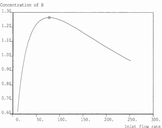
The system illustrated has been designed with the maximum conversion of
product B for the nominal conditions, and is operated at a steady-state point
to control the concentration of B, Cb, by manipulating the inlet flow rate, F.
Although the process seems good from an economic point of view, it exhibits
multiple steady-state behaviour as shown in Figure 1.2 which shows th at more
than one set of inputs exist for the same set of outputs, known as input multiplic
ity. The input multiplicity behaviour can cause control difficulties subject to the
changing operation conditions, such as the changes of disturbances and setpoints.
Thus, there are questions arising while assessing the ability to keep the process
at the desired level in the face of the changing conditions. This attribute of a
system is termed controllability.
• How well can the process be controlled or is it a difficult control problem?
• How many variations in the set point change of the conversion of product
B can the process actually tolerate?
• If the concentration of the reactant A is considered as a disturbance, how
many changes in the disturbance can the process reject successfully?
and moreover
• How can the process be improved if it is not satisfied with the control
requirements?
Such questions are clearly im portant, not only for examining and quantifying how
controllable a process is, but also, more generally, for screening or comparing the
process design alternatives at the process design stage.
Input multiplicity is one complex phenomenon th a t is encountered in chemical
processes, and has been identified as a main cause of destabilisation of the control
systems (Koppel, 1982; Dash and Koppel, 1989). Input multiplicity poses limi
tations on achievable dynamic performance and proves the need for complexity
of control design (Morari, 1983; Skogestade and Postlethwaite, 1996; Sistu and
Bequette, 1995). For instance, with reference to Figure 1.2, there exists no fixed
feedback controller th a t can stabilise both a pair of steady-states 1 and 2, since
the steady-state solutions 1 and 2 have different qualitative behaviour (i.e. dif
ferent gain signs). A conventional controller with integral action only keeps one
of these two steady states stable, and will become unstable for another because
the sign change in the process gain causes the control system from the negative
feedback system to a positive feedback one. Therefore, such a characteristic of
the process should be identified and eliminated or avoided in the process design
O
.8
0.7
150 I n p u t . F ( l / h )
Figure 1.2; Steady-state solution relationship between input and output
Studies in the literature have been shown th at the design of a process de
termines controllability and a controller only ensures the achievable performance
(Morari, 1983; Skogestad and Postlethwaite, 1996). So, it is quite necessary to
have a rough idea of what the inherent properties of the process are and how easy
the process is to control at an early design stage. Controllability analysis could
obtain insights into what the inherent properties of a process are and how they
present limitations on the control performance of the process. Analysing the ef
fects of these limitations early enough in the process design allows the opportunity
to modify the design should the effects be critical to the dynamic performance
of the process (Perkins et a/., 1996). Modifications of a process design itself,
such as changing inputs or outputs, operating points, values of design parameters
and even structure, can sometime affect the dynamics of the process significantly
more than changes in the controllers (Morari, 1983).
Consideration of the controllability of a process at the very early phase of
the process design is now being widely accepted in both academia and industry,
Chapter 2). A growing amount of evidence points to the desirability of incorpo
rating controllability consideration into all phases of the process design. It may
be better in the long run to establish a process th a t has higher capital and energy
costs if the process provides more stable operation and achieves less variability
in product quality. A number of relevant techniques have been proposed, in
cluding optimisation-based approaches (Luyben and Floudas, 1994; Perkins and
Walsh, 1996) and bifurcation-based analysis and design (Morari, 1992; Russo and
Bequette, 1996, 1998).
In this thesis we present an approach to modifying a process design for im
proving controllability, using bifurcation analysis and optimisation. Bifurcation
analysis, a method for studying how qualitative behaviour of a nonlinear system
changes as the parameters vary, is recognised as a powerful tool in nonlinear
system analysis and widely applied to chemical processes (Aris, 1979; Seider et
a i, 1991; Sistu and Bequette, 1995). Morari (1992) suggested th a t bifurcation
analysis should be employed in controllability analysis for nonlinear systems. Bi
furcation analysis could be sufficient to obtain a qualitative picture of the solution
space for a nonlinear process as a param eter of the process varies at the design
stage when there is only limited information available. This can be used to iden
tify the potential control difficulties determined by the process design, and to
investigate the effects of the design and operating param eters and disturbances
on them, hence providing the guidance to eliminate them by modifying the pro
1.2
Objectives
The primary aim of this thesis is to develop a methodology for modifying an
existing process design with a fixed control structure for improving controllabil
ity over the operating regions in the face of a disturbance. In order to modify
an existing process design for controllability it should be essential to understand
what the potential control difficulties are and how the param eters under consid
eration affect them. Results from this analysis lead to a process modification so
th a t such difficult control problems are eliminated or avoided by adjusting the
design param eter values. The methods presented in this thesis dedicate to these
purposes. The objectives are:
• to develop a methodology, based on bifurcation analysis, for determining
potential control problems associated with inherent characteristics of a non
linear process over the entire operating region of interest and analysing the
param eter effects on these problems, and then
• to determine a method for modifying the process to improve controllability,
while preserving modifications as small as possible.
1.3
Outline of the Thesis
The work in this thesis is broadly divided into two parts: the first part is con
cerned with the development of a new approach to controllability analysis of
nonlinear systems with input multiplicity; the second part presents a static feed
back optimisation formula as a trade-off between controllability and economics
in process design modifications, and the applications of the proposed method to
Chapter 2 serves as a brief literature review and background introduction to
the methods used in this thesis. The main ideas on nonlinear systems, controlla
bility, and bifurcation analysis are given. A brief review on controllability analysis
and design techniques available in the literature is presented, while identifying
potential limitations of these methods for nonlinear systems and addressing why
the bifurcation-based approach as an appropriate one.
In Chapter 3, a new bifurcation-based analysis method for nonlinear processes
with input multiplicity such as this described in Figure 1.2 in §1.1 is described and
applied to an exothermic continuous stirred tank reaction (CSTR) th a t exhibits
multiplicity as an illustrative example. The results are compared with analytical
solutions.
Chapter 4 presents an optimisation-based approach to modifying an existing
process design th a t has control difficulties associated with undesirable dynamic
behaviour determined by the process design. A static feedback optimisation for
mulation is developed th a t can modify the process design to avoid the poor dy
namics in the operating region while minimising changes to the process, namely
producing a feedback optimising design (FOD). An exothermic CSTR as an illus
trative example dem onstrates the features and application of this method.
C hapter 5 presents case studies to dem onstrate the applications of these ap
proaches in chemical processes. Two cases are given: one is a reactor-separator
system including recycle and another is an industrial polymerisation reaction. In
each case study, the control problems associated with the given process design
and control structure are identified and how the input, disturbance and design
parameters influence them is investigated; then the process design modifications
are given; and closed-loop dynamic simulations follow in the final section.
In Chapter 6, the major findings and contributions of the work presented in
L iterature R eview
This chapter outlines the background of this thesis and serves as
literature review. The main ideas on nonlinear systems and the con
cept of bifurcation analysis which is used in this thesis are briefly
introduced. Process inherent limitations on controllability are dis
cussed in the context of perfect control and process inversion. The
relationship between multiplicity and controllability is discussed. A
brief review on controllability analysis techniques and design methods
for design and control available in the literature is presented, high
lighting issues th at need addressing.
2.1
Basic Concepts and Properties of Nonlinear
Systems
2.1.1
F u n d am en tals
S y ste m M od els
In this thesis we consider a continuous nonlinear dynamical system of the form:
x = f { x , u ) , (2.1)
where a: G 5R” is the n dimensional state variable vector, u G % is the m anipulated
variable, and • denotes differentiation with respect to time t. The vector function
/ and its partial derivatives with respect to x and u are assumed to be continuous
functions of x and u.
N o S u p erp o sitio n P rin cip le
The superposition principle states, in general, th a t the response of a linear system
to a sum of inputs is the same as the sum of the responses of the individual inputs.
T h at is, a linear combination of solutions
X = axi + bx2 (2.2)
for a system with the form
X = f { x ) (2.3)
only satisfies the system ( 2.3) if
i.e. only if the system ( 2.3) is a linear one.
The superposition principle for a linear system does not apply to a nonlinear
system.
D ep en d en ce on In itial C on d ition s
The dynamic character of a linear system response to an input change is indepen
dent of the specific operating conditions at the time of implementing the input
change. In other words, identical input changes implemented at different operat
ing steady-state conditions will give rise to output changes of identical magnitude
and dynamic character.
A nonlinear system response to a sum of inputs is not equal to a sum of
the individual responses and the magnitude, and the dynamic character of the
response to an input change are dependent on the initial operation conditions.
A distinguishing characteristic of nonlinear systems th a t makes them differ from
linear dynamic systems is th a t the qualitative properties of nonlinear systems
could change under small perturbations of the system parameters.
2 .1 .2
P ro p er tie s o f S o lu tio n s
S tea d y -sta te Solu tion s
For a fixed u, a steady-state solution x of the dynamical system ( 2.1) is defined
by the equation:
/ ( f , u ) = OG%", (2.5)
i.e. a solution which does not change in time. There are other term s used for the
“steady-state solution” such as “ equilibrium solution” or “stationary point” . In
S ta b ility o f S o lu tio n s
Stability is an im portant concept in system analysis, which is concerned with de
termining whether the resulting transient response ultimately settles and main
tains a new steady-state when an input change is implemented on a system.
Qualitatively, a linear system th a t is described as stable if starting the system
somewhere near its desired operating point implies th a t it will stay around this
point. A linear system is said to be stable if and only if all the poles are in the
left-half plane (LHP). Systems with poles on the imaginary axis are unstable from
the above notion. The poles of a system with state space description:
X = A x (2.6)
is defined as the eigenvalues of the constant m atrix A, i.e. the roots of the
characteristic equation:
d et{sl - A) = 0, (2.7)
where det{-) stands for determinant. More general, the poles of a system with
transfer function G{s) may be loosely defined as the finite values s = p where
G{p) has a singularity (or is infinity). The stability of a linear system can be
determined from its poles (eigenvalues). A linear feedback system is internally
stable if and only if all its closed-loop transfer functions are stable.
For the stability of the nonlinear system ( 2.1), the linearly stable notion is
used, which is defined as follows (Wiggins, 1990):
D e fin itio n 2.1 Suppose all of the eigenvalues of Df { x ) have negative real parts.
Then the steady state solution x = x of the nonlinear equation ( 2. 1) is asymp
totically stable.
by
A steady state point x is non-stable if at least one real p art of the eigenvalues of
D f { x ) is positive.
2.1.3
T h e C on cep t o f B ifu rca tio n A n a ly sis
One can draw conclusions about the local stability or instability of steady-state
points for nonlinear systems based on the stability or instability of the linearised
systems provided none of the eigenvalues of the linearised systems have zero real
parts. The principle difficulty with cases where some of the eigenvalues of the
linearised systems have zero real parts and are structurally unstable. A critical
case occurs if some of the eigenvalues have zero real p art and the other have
negative real parts. T hat means th a t there are some of the eigenvalues crossing
the imaginary axis. Below we provide a very brief introduction to the related
concepts of bifurcation analysis used in this thesis which help to explain what
happens when the critical case occurs. The text book by looss and Joseph (1990)
provides more precise and complete description of these concepts.
The steady state solutions of the nonlinear system ( 2.1) depend on the values
of u. It is often necessary to study the dependence of the steady state solutions
of the system ( 2.1) on the values of u. For generality, let us assume now th a t
w 6 is a parameter and set
a = w G 5Î. (2.9)
The system with the form ( 2.1) becomes
A branch of solutions is defined as a continuous and uniquely dependent a:(a).
Uniqueness means th a t for every fixed a G (cKo, CKi) there exists an e > 0 such
th a t there exists no other solution Xi{a) of equation ( 2.10) satisfying
||a:i(a) - x (a )|| < e. (2.11)
The branch of solutions can be continued in both directions until certain limit
values of the param eter a, say (g;o,û;i), are reached and the uniqueness assump
tion no longer holds for these values. Such critical points will be called branch
points. At the branch points the behaviour of the solutions of the dynamic sys
tem undergoes a qualitative change. This change includes multiple steady-state
solutions, instability of the solutions, limit cycles, and so on. Such a kind of
phenomenon is commonly called bifurcation.
Normally, a gradual variation of a param eter in a system corresponds to the
gradual variation of the solution of the problem. However, there exists a large
number of problems for which the number of the solutions changes abruptly
and the structure of the solution manifold varies dram atically when a param eter
passes through these values. In order to understand how the qualitative behaviour
of a system changes under the variation of the param eter, bifurcation analysis is
introduced. Bifurcation analysis is a method for studying such qualitative changes
in the behaviour of the nonlinear system when the param eters vary.
For the nonlinear system with the form of ( 2.10), if the steady-state x is a.
regular steady-state point where all the parts of the eigenvalues of the Jacobian
m atrix D f { x ) are nonzero, a small perturbation in the param eter will not change
the qualitative behaviour of the system. Bifurcations occur when some of the
eigenvalues approach the imaginary axis in the complex plane. The simplest
0) or a pair of complex conjugate eigenvalues Ai 2 crossing the imaginary axis
(Ai^2 = ±zo;o, cjq > 0). The bifurcation where Ai = 0 is called a fold (turning or
limit point) bifurcation. The bifurcation where A%_2 = Tzwo, wo > 0 is called H opf
bifurcation. These are the most common bifurcations encountered in nonlinear
systems. A fold bifurcation usually is the cause of multiple steady states. Hopf
bifurcations are responsible for the appearance and disappearance of periodic
solutions. The stability of the system must change at each bifurcation point, and
only at such a point (looss and Joseph, 1990).
If the other param eter effects on the bifurcation points are considered, we
have a picture of the solution dependence on the param eters, which is called a
bifurcation diagram. This diagram can be used to determine how the system
behaves under changing conditions, and then could provide a guideline to modify
the system to avoid bifurcations.
Bifurcation analysis can obtain insights into what the dynamics of a nonlin
ear process is and how parameters influence them and is used to investigate the
behaviour of the process in terms of param eter-dependent branches of steady-
state solutions. Several decades ago, bifurcation analysis was applied to chemical
processes. In the 70’s, Aris (1979) applied bifurcation theory to discuss some
complex phenomena in chemical reactors and Chang and Calo (1979) presented
an bifurcation-approach to determining the regions of unique and multiplicity
solutions to chemical reaction. Recently, bifurcation analysis is recognised as a
powerful tool and widely applied to nonlinear chemical process analysis (Seider
et al, 1991; Pinto et al, 1995; Russo and Bequette, 1996, 1997, 1998; Pushpa-
vanam et al, 2001; Zhang and Henson, 2001). Using bifurcation analysis was
also suggested in process design (Seider et al, 1991; Morari, 1992). Bifurcation
analysis to aid in redesigning processes has been proposed (Russo and Bequette,
The continuation technique, a numerical technique to obtain one or more
branches of steady-state solutions mutually connected at bifurcation points, has
been developed and is widely used for bifurcation analysis (Keller, 1977; Kubfcek
and Marek, 1983). W ith advanced computational techniques and com puter’s
power, continuation and bifurcation analysis software packages available, such as
AUTO (Doedel et aL, 1998), can allow one to carry out bifurcation analysis for
large nonlinear systems.
2.2
The Concept of Controllability in Process
Engineering
Qualitative changes of nonlinear processes resulting in the complex behaviour
have been briefly discussed in last section and bifurcation analysis provides a
method for exploring the complex solution spaces for a nonlinear process as a
param eter of the process varies. W hen a nonlinear process exhibits complex
characteristics, the control performance of the process might be adversely affected
or possibly the process cannot be controlled. This section is concerned with the
issue of controllability, which describes the achievable dynamic performance (set
point following and disturbance rejection) for a process in control.
In the literature, there are many different definitions about controllability.
Ziegler and Nichols (Ziegler and Nichols, 1943) first defined controllability as
“the ability of the process to achieve and maintain the desired equilibrium value” .
Later the term “controllability” became synonymous with the rather narrow con
cepts of state controllability, which was introduced by Kalman in the 60’s. State
controllability is defined as the ability to bring a system from a given initial state
criterion for controllability in the control system community but not necessarily
the most appropriate for chemical process control. This is because state con
trollability is concerned only with the value of the states at discrete values of
time, while in most cases we want the outputs to stay close to some desired val
ues (trajectory) for all values of time, and w ithout using inappropriate control
inputs.
An alternative is functional controllability, defined by Rosenbrock (1970). A
system with polynomial transfer function m atrix G(s) is called functionally con
trollable if it satisfies the following condition (Rosenbrock, 1970). Given any
trajectory output which is zero for time ^ = 0 and which satisfies certain smooth
ness conditions, there exists an input trajectory u defined for time ^ > 0 which
generates the output y from the initial condition 2 (0) = 0 .
Rosenbrock stated th a t a system with transfer function G{s) is functionally
controllable if and only if G{s) is nonsingular. Sufficiency of this condition is
obvious because the expression
u(s) = G-^y{s) (2.12)
has input trajectories which generate the required output trajectories.
Functional controllability has some advantages over state controllability for
the evaluation of controllability of chemical process as indicated in Russell and
Perkins’ paper (1987). State controllability does not guarantee th a t it is possible
to independently specify arbitrary trajectories of the selected set of output vari
ables, whereas functional controllability does (subject to smoothness conditions).
This is im portant since the main goal of regulatory control is usually to maintain
the plant at some steady state.
satisfactorily though they are not (state) controllable” . An example of tanks in
series was given by Skogestad and Postlethwaite (1996). As the result of this
example, it is seen th a t the property of state controllability may not imply th a t
the system is controllable in a practical sense.
Functional controllability depends on the invertibility of the transfer function.
Thus an examination of the properties of the system which prevent the inversion
of the system will provide a valuable tool for controllability analysis and therefore
control system synthesis.
To avoid confusion with state controllability, Morari (1983a) also introduced
the concept of ^''dynamic resiliences^ which describes the quality of control be
haviour th a t can be obtained for a plant by feedback. This term does not capture
the fact th a t it is related to control design.
Recently, the concept of input-output controllability is introduced. Skogestad
and Postlethwaite (1996) defined the input-output controllability as “the ability
to achieve acceptable control performance” and then followed an explanation
“to keep the outputs (y) within specified bounds or displacements from their
references (r), in spite of unknown but bounded variations, such as disturbances
(d) and plant changes, using available inputs (u) and available measurements
(ym) and (d ^)” .
The input-output controllability definition is more in tune with most engi
neers’ intuitive feeling about what controllability means, though only a structural
property of a process is involved. In particular, for instance chemical processes,
there are a lot of bounds, such as inputs, measurements, devices, and disturbances
and uncertainties, and chemical processes are likely to exhibit strong nonlinear
and complex behaviour subject to changing operation conditions and uncertain
ties. In this sense, the general notion of controllability, which follows the Skoges
as controllability.
Often the controllable performance of a system is assessed by exhaustive sim
ulations, which requires a specified controller design. This implies th a t it is not
possible to know from this kind of assessment if the behaviour is a fundamental
property of the system, or if it is due to a specific controller used. By definition
controllability does not depend on the controller but only on the system itself.
A potentially rigorous approach to controllability analysis is an optimisation-
based test th a t formulates mathematically the control objectives, the class of
disturbances, the model uncertainty, etc., and then attem pts to synthesis ideal
control to see whether the performance objectives can be met (Perkins and Walsh,
1996). This could be applied to processes w ithout detailed control designs on
controllability assessment and much progress has been made in this area (see
§ 2.5.3).
So, there are many different ways to definite and assess the controllability of a
process. W hat is ultim ately of interest is the dynamic performance of the process
subject to disturbances, model param eter and operating condition changes, and
other changes in its environment, and what is more desirable is to have a few
simple tools which can be used to obtain a rough idea of how easy the process
is to control. The methods should be independent of detailed controller designs
so th a t the inherent limitations on controllability by the process design itself,
which no control system, whatever sophisticated, will be able to overcome, can be
identified; and the methods should enable to effectively analyse the effects of these
limitations, which could lead an modified process with improved controllability. It
is some of importance, as stated by Perkins et a i (1996), th a t analysing the effects
of these limitations early enough in the design process allows the opportunity to
This thesis will focus on developing an analysis methodology for process mod
ifications, rather than only for controllability evaluation as the m ajority work had
been concerned with in this area.
2.3
Limitations on Controllability
Controllability describes the achievable dynamic performance of a process inde
pendent of controller design. In order to analyse controllability, it is desirable
to understand what imposes limitations on controllability and how the process
behaves subject to changing conditions. It has been identified th a t some process
characteristics will limit the control performance and pose control difficulties for
controller design, such as input constraints, time delays, right half plane (RHP)
zeros, and a number of techniques are now available to evaluate their potential
impact on closed-loop performance mainly for linear systems (see Morari, 1983;
Skogestad and Postlethwaite, 1996).
In this section the limitations on the control performance and difficult control
design problems associated with the inherent characteristics of a process such
as RHP zeros are addressed. Several concepts related to control system design
and analysis are given. The definitions and ideas for linear systems are briefly
described in order to explain the nonlinear approaches for nonlinear systems.
2.3.1 T h e C o n cep t o f Zeros and Zero D y n a m ic s
A controller generates an approximate inverse of the process in an implicit or
explicit form (Morari, 1983). This implies th a t the inverse characteristics of the
process will determine if the control is easily realised or not. In order to study
the inverse behaviour of a nonlinear process, the concept of zero dynamics is
Z eros
For a single input single output (SISO) linear system with input-output transfer
function G{s), the zeros Zi are the solutions to G{zi) = 0, as in the following
definition:
D e fin itio n 2.2 (Zeros) The zeros of a linear system with the state space form:
X = A x + B u (2.13)
y = C x (2.14)
are the roots of the numerator polynomial of its transfer function:
G(s) = C { s I - A ) - ^ B
G a d j ( s I - A ) B d e t{sl — A)
i.e. the roots of C adj(sI-A )B (Kravaris and Kantor, 1990a).
(2.15)
The definition of zeros is based on a transfer function description, which is a
minimal realisation of a system.
There will be additional zeros found if the description is not minimal. Those
additional zeros arise from hidden pole/zero cancellations in the non-minimal
order description. A minimal order realisation of the system will, however, lead
to the same zeros as the transfer function description (Kravaris and Kantor,
1990a).
For a multivariable system, the following definition of the zero of a multivari
D e fin itio n 2.3 (Zeros) The zeros of a linear multivariable system,
X = A x + B u,
y = C x, (2.16)
are the roots of the determinant of its transfer function matrix, i. e.
\Cadj{sI - A )B \ = 0, (2.17)
where the transfer function matrix is square (MacFarlane and Karcanias, 1976).
When the transfer function m atrix is not square, it is no longer possible to
definite the zeros in terms of determinants. The more general definition of the
zeros of a multivariable system resulting from the generation of the notion of the
determinant of a square m atrix is expressed as: those values of s for which the
rank of the transfer function matrix G{s) is reduced are called the zeros of G{s).
R e m a rk 2.1 It is possible fo r a multivariable system to have poles and zeros
in the same location. In evaluating the zeros of a multivariable system from the
determinant of its transfer function matrix, it is therefore utmost important to
ensure that the denominator polynomial contains all the system poles, i.e. ensure
that there has been no pole-zero cancellation when form ing the determinants (see
Morari and Zafiriou, 1989).
An alternative interpretation of the zeros of a system is to view them as
the poles of the inversion of the system. This view makes it easier to move to
Z e ro D y n a m ic s
For a linear system, the zeros are the roots of num erator polynomial and, in
other words, are the poles of the inverse of its transfer function. The zeros of
a linear system are completely determined by the characteristics of its inverse.
For a nonlinear system, transfer function, on which linear system zeros are based,
cannot be defined, and therefore cannot have zeros as a set of numbers. A notion,
zero dynamics^ is imported, which is analogous to the right half plane (RHP) zeros
of a linear system. The zero dynamics for a nonlinear system is defined to be the
internal dynamics of the system when the system output is kept at zero by the
input (Isidori, 1995; Slotine, 1991). In order not to disrupt the whole flow of this
thesis, the more details about zero dynamics is given in Appendix B.
Regarding the stability of the zero dynamics, the terms of the minimum phase
(MP) and nonminimum phase (NMP) are used and defined as:
D e fin itio n 2.4 A system is termed m inim um phase (MP) at a steady state point
X i f its zero dynamics are stable at x, otherwise, it is nonm inim um phase (NMP).
2 .3 .2
P erfect C ontrol
P e rf e c t C o n tro l o f L in e a r S y ste m s
Let the process model be:
y — G u Gd d, (2.18)
where G and Gd are the process and disturbance transfer functions, respectively.
“Perfect control” is achieved when the output is identically equal to the reference,
i.e. y = y ref- To find the corresponding process input, let us set y = y ref and
solve ( 2.18) for u:
which represents a perfect feedback controller, where G~^ is the inverse of the
process. When proportional feedback control
u = K { y r e f - y ) (2.20)
is used, we have the form:
u = {I + KG)-^Kyref - (/ + KGY^KGdd. (2.21)
If we make K “large” then we see qualitatively th a t ( 2.21) becomes
u ^ G ^yref — G ^Gdd. (2.22)
An im portant lesson therefore is th a t perfect control requires the controller to
somehow generate an inverse of G (Morari, 1983). From this perfect control
cannot be achieved if
• G contains RHP-zeros (since then G~^ is unstable);
• G contains time delays (since then G~^ contains a prediction);
• G has more poles than zeros (since then G~^ is unrealizable).
P erfect C ontrol o f N onlin ear S y stem s
Consider a nonlinear system with the following form:
X = f { x , u ) , (2.23)
where x G u G 5R, denote the state variable vector and the manipulated
variable, respectively, and f denotes smooth vector fields on 9%"^, h is a smooth
scalar function on 5ft. The system ( 2.23) can, more generally, be described by
the in p u t/o u tp u t nonlinear operator implied by the model:
y = P M , (2.24)
where P is a general nonlinear operator th a t maps the input u into the output,
or response, y. If ÿ represents the actual measurement of the plant output then
the model error obtained as
e = (2.25)
enables us to express
ÿ = P[u\ + e (2.26)
as the relationship between the input and the actual plant output.
Given y^e/ as the desired trajectory for the actual plant output y to follow,
the control action u th at satisfies the objective
mm = Wyref ~ ÿ\\ (2.27)
is obtained as
u = P~^[yref - e], (2.28)
provided th a t the inverse of P~^ exists. If yref is selected as the set-point yset for
2/, then
u = P ~ ^ [ y s e t - e\. (2.29)
( 2.29) implies an open-Ioop control policy, and feedback appears only in the
presence of the existence of the error, i.e. e ^ 0.
It is clear th a t ( 2.29) results in so called “perfect control” when P~^ exists
(and is realisable). For an nonlinear operator the P~^ may not exist. If this is
the case, it cannot be realisable. For nonminimum phase systems, the problem is
analogous to the linear case; the inverse of a time delay system is not realisable
due to the necessity of producing predictions.
2.3 .3
Id eal ISE O p tim al C on trol
As stated in the previous section, perfect control is not possible for all systems.
A way to have insight into the “best” control performance is to consider an ideal
controller which is integral square error (ISE) optimal. For invertible system, this
is equivalent to considering perfect control as above, but for non-invertible sys
tems this approach makes it possible to determine the “best” possible controller
(in terms of ISE). For a given output trajectory (which is zero for time t < 0),
the ideal controller is the one th a t generates the plant input u{t) (zero for time
^ < 0) which solves the following;
1 r,
m m I S E = - j ^ \ \ y r . i - y \ \ \ (2.30)
subject to
X = f { x , u ) , (2.31)
y = h{x),
where u is the input, y is the output, x is the state vector, yref is the reference
output, / and h are the plant model equations, and Xq is the vector of the initial
states. This controller is ideal in the sense th a t it may not be realisable in
practice because the cost function includes no penalty on the input u{t). The
perfect control { I S E = 0) represents the inverse of the process.
For a SISO stable plant with real RHP zeros at Zi,i = 1, ...,m , the ideal ISE
value for a step change in the reference is given by (Morari and Zafiriou, 1989):
m 2
I S E = (2.32)
2=1
or with complex RHP zeros z = x ± j y
4x x^ + y^
I S E = -. (2.33)
Thus, as for SISO linear systems, RHP-zeros close to the origin imply poor
control performance. Therefore, to relocate the zero positions can improve the
control performance (Skogestad and Postlethwaite, 1996).
R e m a rk 2.2 For a MIMO linear plant with RH P transmission zeros at Zi, the
ideal IS E value fo r a step disturbance or reference is also directly related to ^
(Qiu and Davison, 1993).
For nonlinear systems having nonminimum phase behaviour the problem ( 2.31)
cannot be solved numerically due to two m ajor problems:
• An infinite time horizon is not implement able in a nonlinear setting
• The solution I S E = 0 (a representation of the inverse of the process) is
Thus unstable zero dynamics impose unavoidable limitations on the closed-loop
performance of nonlinear systems (Seron et ai, 1997).
2 .3 .4
C on trol P ro b lem s A sso c ia te d w ith U n s ta b le Inver
sion
Unstable inverse behaviour of a system has been identified as one of the system
inherent limitations on control performance. Such a characteristic also presents
hard problem for the stability of the controller. Concerning the realisation of a
controller for a linear system RHP zeros contribute additional phase lags to the
system when compared to th a t of a minimum phase system with the same gain. A
larger phase lag brings the system closer to its stability margin (Stephanopoulos,
1984). The extra phase lag also causes a limited speed of response by limiting the
obtainable bandwidth. The upper bound on the bandw idth lu for a SISO system
is approximated by w < z /2 (z is a real RHP zero) (Skogestad, 1996).
For the control of a nonlinear system with NMP behaviour has a similar effect
(Seron et al, 1997). The presence of unstable zero dynamics forbids the imple
mentation of any controller from the class of nonlinear inversion-based controllers
since such a controller is unstable.
R e m a rk 2.3 A NM P system could be stabilised either with longer prediction
horizons or by putting a penalty on the input in the objective function within the
framework of optimal control such as nonlinear model predictive control (NMPC).
However, an off set-free performance (i.e. ideal optimal control) cannot be achieved
in the presence of a disturbance when the input is penalised in the objective func
I
3B
2
!
CO
Steady state input
Figure 2.1: Two possible types of multiplicity, a) input multiplicity; b) output multiplicity.
2.4
Input M ultiplicity and Controllability
In the previous sections, we have discussed difficult characteristic of a system
with respect to the closed loop stability and performance. A stable and invert
ible process is very desirable from a control design standpoint. However, for a
nonlinear process, the characteristic behaviour of the system and its inverse such
as stability may change with changes in operating conditions, resulting in difficult
control problems.
A multiple steady-state phenomenon, namely multiplicity, is often found in
nonlinear chemical processes, which shows multiple solutions and changes in the
stability of the solutions. Chemical processes have been known to exhibit such
nonlinear behaviour. A number of the papers published have reported multiplicity
found in reactions, distillation columns, polym erisation reactions, etc. (Amund
son and Aris, 1958; Uppal et a i, 1974; B alakotaiah and Luss, 1981; Dash and
Koppel, 1989; Gani and Jprgensen, 1994; Sistu and B equette, 1995; Ray and
Villa, 2000).
multiplicity and output multiplicity. Input multiplicity refers to the case where
there exist more than one steady state solutions when the output is specified
(curve (a) in Fig. 2.1); output multiplicity, the most common form, refers to the
case where one input can produce more than one distinct outputs (curve (b) in
Fig. 2.1).
Uppal et al. (1974) and Aris (1979) have presented multiplicity behaviour
found in chemical reactors and Koppel (1982) have studied the effect of input
multiplicity in control systems. Dash and Koppel (1989) have shown a number of
chemical process examples with input and output multiplicity and dem onstrated
th a t input multiplicity can be a main cause of “sudden destabilisation” of the
controlled system with integral action. Recently, Sistu & Bequette (1995) and
Seki & Morari (1998) demonstrated the control performance and control prob
lems imposed by input multiplicity behaviour under nonlinear model predictive
control (NMPC). A process having input multiplicity behaviour is difficult to con
trol because there exists more than one steady state m anipulated variable value
associated with a given output. A process with input multiplicity behaviour also
places a limitation on the structure of the feedback controller (Koppel, 1982)
and poses the feedback performance limitations since there must exist unstable
zero dynamics on one “side” of the steady-state operating curve under some mild
assumptions (Russo and Bequette, 1996). Therefore, the attention in this thesis
2 .4 .1
In p u t M u ltip lic ity and R H P Zeros
In this subsection the combination between input multiplicity and RHP zeros or
zero dynamics of processes will be discussed. It has dem onstrated for SISO sys
tems th at models having input multiplicity behaviour will, under some assump
tions have RHP zeros (Sistu and Bequette, 1995). This implies th a t a process
with input multiplicity will have stability changes in its inverse.
Consider the SISO continuous nonlinear system w ith the form ( 2.23). The
steady state solution to the system ( 2.23) is obtained by solving the equations
of the form:
0 — (2.34)
ys = h(xs), (2.35)
where the subscript s indicates steady state values.
If the equation ( 2.35) has multiple steady-state solutions then the steady-
state input-output relationship could be depicted by the curve (a) or (b) shown
in Figure 2.1. A process having output multiplicity can reach a nonunique output
ys for a given input depending on the initial conditions. On the other hand,
a system with input multiplicity behaviour can have more th an one steady-state
input Us for a specified output It is noted from the curve (a) th a t the steady-
state gain changes its sign in the operating region.
Mathematically, the condition for the existence of the steady state input mul
tiplicity is (Koppel, 1982):
G(0) = - C A - '^ B = 0, (2.36)