Analysis of Pollard's Rho Factoring Method
Soud K. Mohamed
NTNU (Nowegian university of Science and Technology) Corresponding: [email protected]
Abstract. A comprehensive heuristic analysis of the Pollard’s Rho Method
(PRM) is given. The analysis is based on ultimate periods and tails dis-tribution of sequences. Ifnis the composite number to be factored, then an improved version of PRM is developed which has an expected run time ofO(√8nlnn) on a multi-core architecture which utilized a clever way of
evaluating polynomials.
Keywords:ultimateperioddistribution; parallelization; taildistribution
Introduction
The security of cryptographic schemes based on RSA, the most widely used cryptosystemforsecuredatatransmissiononthe Internet,reliesonthe factorization of large integers. Hence integer factorization algorithms must play a very importance role insecure communication onthe Internet.
Thereareseveralalgorithmsoffactorizingintegers,themostcommonones being: trivial division, Pollard’srho and (p−1)methods,Fermat’smethod, Index calculus method, Elliptic curve method, Quadratic sieve method and number field sieve method. A good survey of modern factorization method is given by Lenstra [12]. Good analyses for most of the methods are found in the literature [1, 2, 3, 12, 16]. Trivial division is the most inefficient one of all the factorization methods. To find a factor p of a composite√number
n bytrivial division, one needs to divide n byall primesless than n. The best factorization algorithm so far is the number field sieve, which has sub-exponentialrun timeasindicatedbyLenstra[12]. ThePollard’srhomethod has a heuristic expected run time of O(√p), where p is the smallest factor of a composite number n [2, 3, 11, 12].
Pollard’s rho method is one of the earliest factoring method in contem-porary world which was developed by Pollard [14]. Since is invention in the seventies, there are very few analyses found in the literature: the well-known heuristic analysis based on the Birthday Paradox and the analysis which determining the probability of success discussed by Bach [2]. This paper proposed a new analysis of PRM, which is based on ultimate periods and
1
tails distribution of sequences in Zp. An improve parallel implementation of
PRM is proposed, which has expected run time O((lnp)√4 p).
Let pbe a prime number≥5 and f(x) be a polynomial function over Zp,
and ak =f(ak−1) be a sequence inZp. Fixing a choice of coefficients off(x),
then the average of the ultimate periods of ak as a0 runs over all element
in Zp is called the ultimate period of f with respect to p, and is denoted
by upp(f). We conjecture that for a polynomial f(x) ∈Z[x] which is not a permutation, we have that upp(f)≤√p.
If ak = f(ak−1) is a sequence, then Floyd Cycle Detection Algorithm
(FCDA), as explained by Pollard [14] and Brent [3], picks every other element in ak by using the (sub)sequence bk = f2(bk−1), where b0 = a0. Every
sequence in Zp is ultimately periodic, hence it has a tail. The presence of
tail makes the use of FCDA algorithm to detect collision inevitable as one is not sure when the sequence will enter a circle. With an appropriate selection of sequence generator, we show that the distribution of of the tails can be approximated by the function ln(p)√4p. This can be used to improve the run
time of PRM.
On the other hand, if the period of the sequence ak is even, them
applica-tion of FCDA reduces it by half. Referring to original FCDA as the FCDAof
index 2, one can introduce an FCDA of index t. Then using the algorithm,
the period of ak is reduced by a factor of t, provided t divides the period
of ak. We show that by utilizing suitable FCDA of length t, one can obtain
sequences bk with expected period ln(p)4 √
p.
Parallel implementation of factoring algorithms have been use in order to increase the efficiency of factoring algorithms [5, 6, 7]. For the PRM, two parallel implementation have been consider which have run time of O(√p) and O(√p(logm)2/m) [6, 7]. An improved parallel implementation which
with the help of fast polynomial multiplication is proposed.
A brief review of the literature is given in Section 1, while in Section 2 an investigation of ultimate periods of some special sequences and subsequences is discussed. In Section 3, the analysis of PRM is provided together with an improve parallelization of PRM. Finally conclusion and further research areas are given in Section 4.
1. Literature Review
In this section a literature review of the PRM analysis is given. Also a brief review of fast polynomial evaluation algorithms and it runtime is provided.
1.1. Pollard’s Rho Factorization Method. Letn be a square-free com-posite number, and let p be the smallest prime dividing n. If one picks numbers a0, a1, a2, ... from Zn independently at random, then after at most
that ai ≡as modp. Since n is composite, there is another prime factorq of
n withp < q such that xi 6=xs mod qwith probability at least 1−1/q even
when ai ≡as modp. Hence qmust divide n, and so gcd(n, ai−as) =q is a
non-trivial divisor ofnwith probability 1−1/q. The fact thatai ≡as modp
fori < swill be referred to ascollision. By using the Birthday Paradox, the expected number of cycles before one encounters a collision is roughly of the order of √p. This briefly explains the Pollard’s Rho Factorization Method (PRM).
To generate a random sequence, a ”random” function f on Zp is used.
Since all function on Zp are polynomials, a polynomial f(x) which is not a
permutation polynomial can be use as a random map. The so called magical polynomial f(x) = x2+c, wherec6= 0,−1,−2 are widely used. The current
analysis of the algorithm work under the assumption that f(x) behave like a random function which has never been proved!
To find a factorpof composite integernby PRM, a Floyd Cycle Detection Algorithm (FCDA) is used. The algorithm simultaneously compute ak =
f(ak−1) and bk = f(f(bk−1)), where b0 = a0 and check whether gcd(aj −
bj, n) > 1 for some j > 0. In that situation we would have encounter
a collision modp. The algorithm can be improved by accumulating the differences aj−bj and compute the gcd in a batch, that is, by letting zj =
Ql
j=1aj − bj and compute gcd(zj, n) only when l is a multiple of m for
log2n ≤m≤√4n as shown by Pollard [14].
1.2. Analysis of PRM in the literature. As stated in the introduction the most well-known analysis of PRM found in the literature are the one based on the Birthday Paradox. Pollard [14] heuristically established that a prime factor p of a composite number n can be found in O(√p) arith-metics operations. The heuristics was based on the fact that the generating sequence, which was then the polynomial x2+c for an integerc6= 0,2, is a
random polynomial chosen among thepp. The first rigorous analysis of PRM
was done by Bach [2], who showed that the probability that a prime factorp
is discovered before thekth iteration, forkfixed, is at least (k
2)/p+O(p −3/2).
The original PRM uses FCDA to determine collision. Brant [3] proposed another cycle-finding algorithm which is on average about 36 percent faster than FCDA. He used his algorithm to improve PRM by about 24 percent. The improvement was obtained by omitting the termsaj−bj in the product
zj ifk <3r/2, where ris the power of 2 less than or equal to sum of the tail
and period [3, sec. 7]. However to find a r one has to find a cycle first!
Parallel implementation of PRM method was discussed by Brent [5]. He showed that if one uses mparallel machines, the expected heuristic run time of PRM is O(
√ p √
m), a nonlinear speed up! Crandall [7] came up with a new
in a heuristic time of O((log2m)2 √
p
m ). However, the heuristic has never been
tested as noted by Brent [5].
1.3. Fast Polynomial Evaluation. Two type of fast polynomials evalu-ation are found in the literature. Sequential implementevalu-ation uses a single core architecture, while parallel implementation utilizes a multi-core archi-tecture. The well-known Horner’s method, which is sequential, is often the default method for evaluating polynomials in many many computer libraries as noted by Reynolds [15]. The method has a runtime of O(m), where m is the degree of the polynomial. There are two parallel algorithms which are the most common. Dorn’s method, which is a generalized form of Horner’s form, and has a run time of at least 2m/k+ 2 log2k, wherek is the number of processors as indicated by Munro, Paterson [13]. The other one is Es-trin’s algorithm, also explained by Munro et. al. [13], which has run time of
O(log2m), hence is very suitable for polynomial whose degree is a power of 2. The later was also discussed by Xu [17] and Reynolds [15].
2. Preliminaries
In this section we special sequence in Zn and their properties, as well as
the relation between sequence in Zn and those in Zp for a factor pof n.
Definition 2.1. [3, 8] A sequence ak is a ultimately periodic if there are
unique integers µ≥ 0 and λ ≥ 1 such that ak =ak+λ for each k ≥ µ. The
number λ is called the ultimate period or period of the sequence, while the number µ is the tail or prepedriod of the sequence. The sum λ+µ is the
length of the sequence.
Example. The sequence ak : 1,2,5,3,10,9,13,9,13,9,13,9,13,9,13 is
ulti-mately periodic of ultimate period 2, tail 5 and length 7.
Let p be an odd prime. Then any natural sequence in Zp is eventually
periodic, since Zp is a finite set. Consider a polynomial function f(x) over
Zp. Ifaj ∈ Z∗p, then the sequence ak =f(ak−1) is called the sequence in Zp
generated by f(x). Now if t be a positive integer, then bk = ft(bk−1) is a
subsequence ofak. Note that the subsequencesbk defined above are obtained
by picking every t-th element of ak.
Example. Consider the sequenceak : 1,2,5,3,10,9,13,9,13,9,13,9,13,9,13.
Then bk : 1,5,10,13,13,13, ... and bk : 2,3,9,9,9, ... are subsequences of ak
of ultimate period 1.
Consider the sequencesak =f(ak−1) inZp generated by polynomialf over
Zp, and their corresponding subsequences bk = ft(bk−1) for some positive
integer t. Then the ultimate periods ofak and bk are related as shown in the
Lemma 2.2. Letak =f(ak−1)be a sequence inZp generated by a polynomial
f over Zp with ultimate period λ and let bk = ft(bk−1) for some positive
integer t be a subsequence with ultimate period δ. Then
i. δ divides λ, and
ii. δ =m/gcd(λ, t).
Proof. i. bkis obtained by picking elements with indices 0, δ,2δ,3δ, . . .. Since
δ ≤λ and bk is ultimately periodic, it follows that δ|λ.
ii. Since the sequences are ultimately periodic, there is an integer s such that a0 = bδ = asλ = aδt, so that sλ = δt, which implies that δ = t/sλ . We
claim thatt/s= gcd(λ, t). Ift/s=g, then observe thatg|λ, sinceδis indeed an integer. On the other hand λ =δg, so that sδg =δt, which implies that
t =sg. Hence g is a common divisor of δ and t. To show that g = gcd(λ, t)
is left as an exercise.
2.1. Ultimate period of a Prime. Let n be a square-free composite in-teger and p a prime factor of n. In this section an investigation of ultimate period of special sequences in Zp is given. Also relationship of ultimate
periods of sequences in Zn and Zp is discussed.
Let f(x) is a fixed polynomial of degree m, then there are about p such sequences ak. So as j runs from 1 to p we get p ultimate periods. Now
if the coefficients of f are chosen at random, then there are pm choices of coefficients, and we get pm+1 ultimate period. The average of these periods might be some thing useful.
Definition 2.3. Let p >3 be a prime, let f(x) be a polynomial over Zp of
degree m and let ak =f(ak−1) be a sequence in∈Zp.
1. The average ultimate period ofak for a given coefficients of f as the
initial seeda0 runs over {1,2,3, ..., p} is called theultimate period of f(x) with respect to p, and will be denoted by upp(f).
2. Then the average ultimate period ofakas the coefficients off and the
initial seed a0 run over {1,2,3, ..., p} is called the ultimate period of p with respect to f(x), and will be denoted by upf(p).
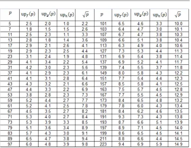
Let f(x) = x2 + 1 , g(x) = f2(x) and h(x) = g2(x). Then the ultimate
periods of f, g and h with respect to the primes pbetween 3 and 225 Figure 1. From the figure we can observe that the ultimate period of a polynomial with respect to a a prime pis a most √p. We have the following conjecture.
Conjecture 2.4. Let p > 3be a prime and let f(x) be a polynomial overZp
which is not a permutation. Then
Figure 1. Ultimate Period for Primes less than 225
Remark 2.5. The ultimate period of a primepwith respect to a polynomialf,
upf(p) is more interesting, because the sound parallelization of PRM found in the literature [5] use random coefficients and initial seeds. However, it exact computation is very time consuming.
Suppose that ak =f(ak−1) for some polynomialf overZp. We determine
the relationship of ultimate period inZnand inZpi fori= 1,2, ..., s. This will
be very useful in the coming sections when we analyze the Rho Factorization Method.
Proposition 2.6. Let n = p1p2· · ·ps be a square-free integer and let ak =
f(ak−1) for some polynomial f over Z. If ak has ultimate periods λ1, ..., λs
respectively in Zp1,Zp2. . . ,Zps, then it has ultimate period lcm(λ1,· · ·, λs)
in Zn.
Proof. It can be easily deduced that the sequence (ak mod p1, . . . , ak modpt)
has ultimate period lcm(λ1, . . . , λs) in Zp1 × · · · ×Zps. Then the result
fol-lows from the fact that Zn ' Zp1 × · · · ×Zps via the isomorphism ϕ :
Zp1× · · · ×Zps →Zn given byϕ(a1, . . . , as) =e1a1+· · ·+esas, where ei are
elements in Zn such that 1 =e1+· · ·+es.
Remark 2.7. The converse of Proposition 2.6 is indeed true, namely if ak
ultimate period λi in Zpi for some i from 1, ..., s. One thing to note here is
that it happen sometimes that all λi are the same!
Remark 2.8. In the next sections, all the analysis will be based on a prime
factor p of a composite n. Although one will be working in n, but because of the classification theory of finite abelian groups, the structure of p inn is kept intact.
3. Analysis of Pollard’s Rho Method
In this section analysis of rho method using tails distribution of sequence
akgenerated by a polynomialf overZp and ultimate period of the sequences
ak is given. The analysis is based on two experiments done the researcher.
3.1. Tail and period distributions. As mentioned in the literature re-view, Brant [3] proposed another cycle-finding algorithm which he used to improve PRM by about 24 percent. The improvement was obtained by omit-ting the terms aj −bj in the product zj if k <3r/2, where r is the power of
2 less than λ+µ [3, Sec. 7]. The motive behind this move was to compute gcd using terms which lie in a cycle. This means that the knowledge of a position in a sequence where a cycle start (the end of the tail) may improve the PRM.
Let n be a composite number and ak = f(ak−1) be a sequence in Zn.
Suppose that λ is a period of the sequence ak = f(ak−1) and µ is its tail.
Then using the help of FCDA, the algorithm PRM finds the smallest prime factor pofn after exactlyλ+µterms.The subsequencebkofak found during
the execution of PRM has ultimate period λ1 =λ/gcd(2, λ) by Lemma 2.2.
Now if FCDA is applied on bk, gcd(bj, b2j) > 1 would be obtained after
exactly λ2 =µ/2 +λ1 terms, and if λ was even, one would need to compute
even smaller number of terms, namely (λ+µ)/2. Hence, applying several FCDA would reduce the number of terms required to get gcd(aj, bj) > 0
even when the order λ is not even, as it would reduce the tail by a power 2.
Remark 3.1. 1. In the original PRM and and its subsequent variants, the
choice bk =f2(ak−1) was preferred only because of computation complexity
of higher degree polynomials. In other word, any power t ≥ 2 would have suffices for successful computation of period of ak, with increased number of
computation as t increases.
2. The nature of the sequencesbkare perfectly suitable for implementation
in computers with t core processors using Estrin’s algorithm. Since the degree 2t, then the algorithm has a run time of O(t).
3.2. Setting up of the experiments. In the first experiment, tails of dif-ference sequences in Zp for different primesp were computed. For the prime
g(x) = f2(x) were computed for all initial seeds a
0 in Zp. For the primes
in the other ranges a sample of size √p was considered. The second exper-iment was conducted to determine the proportion of periods of sequences less than ln(p)√4 p, where p is a prime number. The sequence generator was bk = f2(bk−1), where f(x) = x2 +c. Two instances were used, where the
first instance used random a0 =r0 and c=r2, while the second one utilized
random a0 = r3 and fixed c = f0. For each prime p about √
p tails were computed.
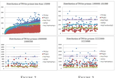
Analysis of Experiment 1. Then tails mean of each primepwith respect to the polynomialsf andg,T Mf(p), T Mg(p), were computed. The the
distri-bution of the TM were than compared toLL(p) = ln(p)·lnp, S(p) =√p, and
LF(p) = lnp·√4 p. Figure 3.2 and 3.2 show comparisons ofT M
f(p), T Mg(p),
LL(p), S(p) and LF(p).
Figure 2 Figure 3
The top left diagram of Figure 3.2 shows that almost all T Mg(p) lies
bellow the function LL(g), S(p), and LF(p), while some of theT Mf(p) are
above the functions. But as p increases T Mf(p) grows faster than LL(p),
but can be fitted into LF(p), while more than half of T Mf(p) lies below
LF(p), see top right diagram. As p moves to seven digits none of T Mg(p)
lies under LL(p), while only a handful of T Mg(p) are under LL(p), see the
bottom left diagram. In the bottom left diagram almost none of tails means are under LL(p), a few of T Mf(p) lies under LF(p), while T Mg(p) can be
approximated by LF(p).
The above analysis draws the following conclusion: If ak = f(ak−1) is a
some positive integert, the expected tail of the sequencebk =ft(bk−1), where
b0 =a0 is ln(p)· 4 √
p with reasonable probability.
Remark 3.2. As p increases LF(p) is moving below T Mg(p), in other word
probability of having a good number of tails below LF(p) decreases. How-ever, in the analysis we used t = 2, so an increase of t will remedy this problem.
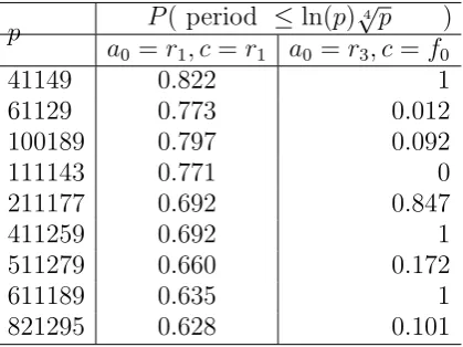
Analysis of Experiment 2. The outcome of the experiment is shown in Table 1. Row two of the table shows probabilities for different primes when
Table 1. Probability of period ≤ln(p)√4p
p P( period ≤ln(p)4
√
p )
a0 =r1, c=r1 a0 =r3, c=f0
41149 0.822 1
61129 0.773 0.012
100189 0.797 0.092
111143 0.771 0
211177 0.692 0.847
411259 0.692 1
511279 0.660 0.172
611189 0.635 1
821295 0.628 0.101
randoma0, care used. They are all greater than 0.5, hence good probabilities.
On the other hand, when the parameter cis fixed (row 3), there are all kind of probabilities, 0, very small and very big.
There are at least few of inferences that can be drown from the table. First, it highlight the concern J. M. Pollard himself raised by Crandall [7] about the consequence of fixing c, as there will be then very few periods O(≤ dlnpe). Moreover, it strengthen the idea of using random parameters
a0 and c in the construction and execution of PRM, as one has a very wide
iterative cycles to work with noted by Crandall [7]. In all the cases considered there were more than ln(p)2 different cycles.
One can then infer that the use of random parametersa0 and care
impor-tant in implementation of PRM, both single and parallel modes. Moreover, ln(p)√4pis a good estimate of the expected period of a sequenceb
kin heuristic
terms.
Remark 3.3. From row 2 one can observe that aspincreases the proportion of
periods less than ln(p)√4 pdecreases. This can be offset by taking appropriate
value of t. Note that in this example t= 2.
inZn, wherec6= 0,−2 is an integer. Chooset such that 2t ≤ dln √
ne. A set of t independently machines will be used and in each one of them, a PRM will be run using the sequences bk =ft(bk−1) for t= 2, ..., t.
The algorithm. Each machine j should perform the following steps:
(1) Set the sequence bjk for j = 2, ..., t, and generate random parameters
a0 and c.
(2) Compute the first M =d√8nln√ne terms, and store the term bj M.
(3) Set N = dln√ne, for l = 0, N,2N, ..., compute the terms bjk for
k > M and store the product
Pl+N = l+N
Y
i=l
(bjM −bjM+i) mod n
(4) Compute gcd(Pl+N, n) . If gcd(Pl+N, n)>1 in one of the machines,
stop. Otherwise, repeat Step 3 until i=M.
Remark 3.4. Observe that the algorithm does not utilize a cycle detection
algorithm in Step 3, instead it computes the difference bM −bM+i for i =
0, ..., M. This move will improve the efficiency of the algorithm as it avoid computation of tow sequences and comparison associated to cycle detection algorithms.
Analysis of the algorithm. The analysis will be based on two implemen-tation, namely a single core architecture and a multi-core architecture. The first thing to note is that the algorithm is a Monte Carlo algorithms, it has a probability of success, which we will try to determine. In Step 2 the algo-rithm is trying to escape the tail and enter a circle, an idea which was use with success by Brent [3]. Using Remark 3.2, Step 2 will reach its goal with a very good probability.
Case 1. For one core architecture, computation of the terms of bk in Step 3
can be estimated as follow. By using the Horner’s form, each term of bk for
k > 0 can be computed inO(ln√n) arithmetic operations, since its degree is less than ln(√n). Step 3 will require O(√8n(ln√n)2) arithmetic operations
from each machine. Apart from computation of bik in Step 3 and 4, there is multiplication of terms and computation of gcd. But it is plausible to consider the cost of only ak and ignore the other. The motive behind this
move is the fact that computation of bk is more costly than multiplication
and gcd computations. Moreover, the cost bound set on bk is the worst-case
scenario, in other word, very few machine will come near the bound. Now the expected cost of each machine isO(√8 nln√n·ln√n+√8nln√n·ln√n) = O(√8 nln√n·ln√n), where ln√n is the cost of computation of terms as in
the sense of [6].
Case 2. Using Estrin’s method on multi-core architecture, each bk in Step
same assumption as in Case 1, the expected cost of each machine is now
O(√8 nln√n), vast improvement from Case 1.
4. Summary and Conclusion
Analysis of Pollard’s rho factorization method is given which is based on the distribution of periods and tails of sequences. An improved paralleliza-tion of the method is given with a run time of O(√8 nln√n). The
paral-lelization can be improved with an improve in the polynomial evaluation algorithms and an increase in the number of cores in a machine.
References
[1] B. R. Ambedkar, S. S. Bedi (2011),A New Factorization Method to Factor RSA Public Key Encryption, IJCSI,90(6.1), 130-155.
[2] E. Bach (1991),Toward a Theory of Pollard’s Rho Method, Information and Compu-tation90, 130-155.
[3] R. P. Brent (1980),An Improved Monte Carlo Factorization Algorithm, BIT20, 176-184.
[4] R. P. Brent (1990),Number Theory and Cryptography, Cambridge University Press. [5] R. P. Brent (1990), Parallel Algorithms for Integer Factorization,Number theory and
cryptography 154, 26-37.
[6] R. P. Brent (1999), Ssome Parallel Algorithms for Integer Factorization, Porc. Eu-ropar’99, Toulouse, Sept 1999.
[7] R.E. Crandall, Parallelization of Pollard-rho factorization, preprint, 23 April 1999 [8] A. Dubickas, P. Plankis (2008),Periodicity of Some Recurrence Sequences ModuloM,
Combinatorial Journal of Number Theory,8, # A42.
[9] G. ESTRIN (1960),Organization of Computer System–The Fixed Plus Variable Struc-ture Computer, Proceedings Western Joint Computer Conference, May, 1960, AFIPS Press, Montvale, N J, pp. 33-40.
[10] A. K. Koundinya, G. Harish, N. K. Srinath, G. E. Raghavendra, Y. V. Pramod, R. Sandeep, P. G. Kumar (2013),Performance Analysis of Parallel Pollard’s Rho Factor-ing Algorithm, International Journal of Computer Science & Information Technology (IJCSIT),5(2), 157-164 .
[11] N. Koblitz (1994),A Course in Number Theory and Cryptography, 2nd Ed., Springer, USA.
[12] A. K. Lenstra (2000),Integer Factoring, Designs, Codes Cryptography, 19, 101-128. [13] I. Munro, M. Paterson (1973), Optimal Algorithms for Parallel Polynomial
Evalua-tion, JCSS, 7, 189-198.
[14] J. M. Pollard (1975), A Monte Carlo Method for Factorization, BIT15, 331-334. [15] G. S. Reynolds (2010), Investigation of different methods of fast polynomial
evalua-tion, Master thesis, The University of Edinburgh.
[16] R. D. Silverman (1987), The Multiple Polynomial Quadratic Sieve, Mathematics of Computation,48(177), 329-339.
[17] S. Xu (2013), Eficient Polynomial Evaluation Algorithm and Implementation on FPGA, Mater thesis, Nanyang Technological University.