Numerical solution of subsonic and transonic flows in 2D and 3D

(1)

Numerical solution of subsonic and transonic ﬂows in 2D and 3D

Jaroslav Huml1,a_{and Karel Kozel}1

1_{Czech Technical University in Prague, Faculty of Mechanical Engineering}

Abstract. This work deals with a numerical simulation of 2D and 3D inviscid and laminar compressible flows around a DCA 18% profile. Numerical results were achieved on non-orthogonal structured grids by the authors’ in-home code with an implemented FVM multistage Runge-Kutta method and an artificial dissipation. The results are discussed and compared with other similar ones (e.g. the results by G. S. Deiwert).

1 Introduction

The authors deal with the development of their own in-home codes that could be applied in general for the simu-lation of any flow, i.e. an inviscid and a viscous (both lam-inar and turbulent) flow, using one or more FVM schemes. In this case the code includes a multistage Runge-Kutta method with a Jameson artificial dissipation and has been successfully tested on the simulation of inviscid and lam-inar flows in a few test cases, i. e. flows in the GAMM channel and in a DCA 8% cascade. Based on the previous successfull use (see i. e. [4] or [5]) authors have decided to apply it for numerical solutions of inviscid and laminar flows around a DCA 18% profile in 2D and 3D, and to verify its general application.

2 Mathematical models

2.1 Navier-Stokes equations

A general two-dimensional flow of a compressible laminar fluid (the authors assumed that the flowing medium was a calorically perfect gas – the Newtonian fluid.) is described by the system of Navier-Stokes equations

Wt+Fx+Gy=Rx+Sy, (1)

where2

W=(ρ, ρu, ρv,e)T,

F=(ρu, ρu2+p, ρuv,(e+p)u)T,

G=(ρv, ρuv, ρv2+p,(e+p)v)T, (2)

a _{e-mail: [email protected]}

2 _ρ_{denotes density of the ﬂuid; (}_u_{, v, w}_{) are components of}

the local velocity respectively in the direction of axis x, y,z;p

is pressure (given by an equation of state);edenotes density of total energy per a unit volume;τi jrepresents shear stress

(assum-ing Stokes Law for mono-atomic gases);qj is heat ﬂux (given

by Fourier’s Law assuming Mayer’s formula);μrepresents dy-namical viscosity;γdenotes the isentropic exponent (equals 1.4 for mono-atomic gases – air); andPris laminar Prandtl number (equals 0.9).

R=(0, τxx, τx_y,uτxx+vτx_y−qx)T,

S=(0, τx_y, τ_yy,uτx_y+vτ_yy−q_y)T

and

p=(γ−1)

e−1 2

u2+v2,

τi j =μ

∂ui ∂xj +

∂uj ∂xi

−1 3δi j

∂uk ∂xk,

(3)

qj=−_γ₋γ 1

μ Pr

∂ ∂xj

p ρ

.

2.2 Euler equations

Assuming an inviscid ﬂuid (μ=0 in viscous ﬂuxesR,S), the system of Euler equations is used instead of the system of Navier-Stokes equations

Wt+Fx+Gy=0 (4)

or in case of 3D simulation

Wt+Fx+Gy+Hz=0. (5)

where

W=(ρ, ρu, ρv, ρw,e)T,

F=(ρu, ρu2₊_p_{, ρ}_u_{v, ρ}_u_w,_(e₊_p)u)T_,

G=(ρv, ρuv, ρv2+p, ρvw,(e+p)v)T, (6) H=(ρw, ρuv, ρuw, ρu2+p,(e+p)u)T,

p=(γ−1)

e−1 2

u2+v2+w2,

2.3 Transformation to the dimensionless form

(2)

system of Navier-Stokes equations3_{(7) is a little di}_ﬀ_erent from aforementioned (1)

Wt+Fx+G_y= Ma∞

Re_∞ (Rx+Sy). (7)

3 Numerical method and scheme

The FVM numerical scheme – the multistage Runge-Kutta method extended by including Jameson’s artiﬁcial dissi-pation to improve the stability of the method4 _{– was} ap-plied to the cell centered form on non-orthogonal struc-tured grids of quadrilateral or hexahedral cellsD5 _{for the} simulation of the ﬂows mentioned previously.

– multistage Runge-Kutta method (RK)

ResW(r)_{i j} = 1 |Di j|

4

k=1

˜

Fr_kΔyk−G˜r_kΔxk

, (8)

W(0)_{i j} =Wn_{i jk},

W(r_{i jk}+1)=W(0)_{i jk}−αrΔtResW(r)_{i jk}+AD(Wn_{i jk}), (9)

Wn+1 i jk =W

(3) i jk,

α0,1=0.5, α2=1,r=0,1,2.

– Jameson’s artiﬁcial dissipation (AD)

AD(Wn_i_,_j)=C1ψ1(Wn_i−1_,_j−2Wn_i_,_j+Wn_i₊₁_,_j) (10) +C2ψ2(Wn_i_,_j₋₁−2Wn_i_,_j+Wn_i_,_j₊₁),

where

ψ1 = p n

i−1,j−2pni,j+pni+1,j

pn

i−1,j + pni,j + pni+1,j

, (11)

ψ2 = p n

i,j−1−2pni,j+pni,j+1

pn

i,j−1 + pni,j + pni,j+1 .

Numerical approximations ˜F,G˜ of convective termsF,G were considered in the forward form of the ﬁrst order of ac-curacy. Numerical approximations ˜R,S˜of dissipative terms R,Swere approximated in the central form of the second order of accuracy and by using dual cells and applying Green’s formula.

The time stepΔtdeﬁned by the stability criterion was computed by

Δt≤ CFL

|u|+a

Δx + |v|+a

Δy +2MaRe∞∞

1

Δx2+_Δy12

.6 ₍₁₂₎

3 _Ma

∞,Re∞is inlet Mach and Reynolds number.

4 _{The scheme and the artiﬁcial dissipation are written for a 2D}

ﬂow, but their 3D forms look similar.

5 _|_D_|_{represents the volume of the cell.}

6 _CFL ₌ _{2 for the multi-stage Runge-Kutta method chosen}

andais the sound speed.

4 Formulation of the problems

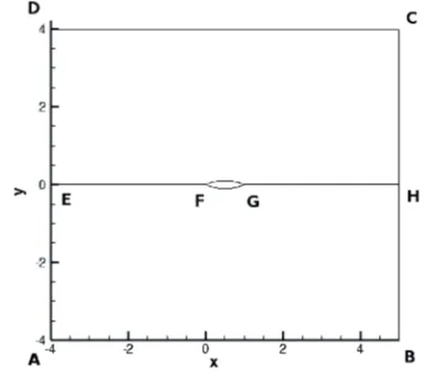
The authors took into account the numerical simulations of 2D inviscid and laminar compressible flows around the DCA 18% profile and around its 3D modification (a sim-ple extension into 3D and aSwept Wingmodification). The outlines of the computational domain are shown in fig-ures 1 and 2. The left and right outlines (AD,BC) and sur-faces (ADLI,BCK J) represent an inlet and outlet of the domain respectively. The bottom and top outlines (AB,CD) and surfaces (ABJI,DCKL) are so calledfree walls, where the same condition was considered similar to at int-let. The symmetry line and plane are divided into two straight lines (EF,GH) and surfaces (EFN M,GHPO) respec-tively, into the parts of the boundary where a symmetry condition was applied. And finally two circular curves be-tween the points (F,G) and two curved surfaces (FGON) represent the bottom/top part of DCA 18% profile – here were prescribed boundary conditions for a solid wall ac-cording to the mentioned type of flow (an inviscid or a vis-cous flow).

In the case of theSwept Wingmodiﬁcation the relative thickness and chord are linearly changed depending on the z-coordinate between (10 %, 18 %) and (0.5, 1.0) respec-tively.

Fig. 1.Geometry of the DCA 18% proﬁle in 2D.

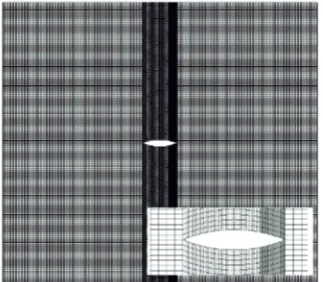
The 2D region and 3D region were covered by three different non-orthogonal structured grids, quadrilateral meshes with 160×160 cells (see figures 3 and 4) and hexahedral grid with 160×160×1 or 160×160×10 cells (see figure 5), where 60 cells were distributed over the DCA 18% profile in thex-direction. The authors made also such a convenient refinement of the mesh around the profile in they-direction for a better detection of viscosity influence in the case of the laminar flows (see figures 4). The smallest spacing was equalled 2/(3√Re_∞).

4.1 Boundary conditions

(3)

Fig. 2.Geometry of the DCA 18% proﬁle in 3D –Swept Wing

modiﬁcation.

Fig. 3.Mesh for 2D inviscid ﬂows – 160×160 cells (grid detail around the proﬁle in the lower right corner).

half – and added virtual cells to these parts from the out-side for a better realisation of all the prescribed boundary conditions (see ﬁgure 6):

– inlet:ρ1=1, u1=Ma1cosα, v1=Ma1sinα, p1was extrapolated from the ﬂow ﬁeld ande1was calculated using the equation of state.

– outlet: p2 was prescribed and the other components were extrapolated from the ﬂow ﬁeld or calculated. – solid wall: velocity components were prescribed so that

the sum of velocity vectors equals zero (viscous ﬂows – u=v=0) or equals zero in their tangential component (inviscid ﬂows – (u, v)n=0).

– free wall: the value of a variable in the cell at the bot-tom/top part of the boundary corresponds to the value at the inlet.

– symmetry: the value of a variable in the top cells of the lower half corresponds to the value in the bottom cells of the upper half and vice versa.

Fig. 4.Mesh for 2D laminar ﬂows – 160×160 cells (grid detail around the proﬁle in the lower left corner and grid detail near the trailing edge in the lower right corner).

Fig. 5.Mesh for 3D inviscid ﬂows – 160×160×10 cells (grid detail of swept wing).

Fig. 6.Application of boundary conditions – inlet and free wall b.c. (stripes), outlet b.c. (ﬁne stripes) and symmetry/solid wall b.c. (light and dark grey).

5 Numerical results and discussion

(4)

num-bersRe_∞ ∈(105_,₁₀7_{) (in laminar ﬂows) and angles of} at-tackα∈(−3◦,3◦).

All the numerical results are presented by using Mach number isolines and isosurfaces, the results for 2D invis-cid flows are shown in figures 7 and 8 and for 3D invisinvis-cid flows are printed in figures 12 (the simple extension into 3D) and 13 (theSwept Wingmodification).

The authors have used the results by G. S. Deiwert [1] for comparison of 2D results and do realize that this com-parison is only informative since our results are not turbu-lent in contrast to Deiwert’s ones. From the comparison of the results it follows that, despite the fact that the authors used a larger number of cells in thex- andy-direction than Deiwert, the minimum values of the pressure coefficient (cp ≈ −0.9, see figure 10) are almost half than the values by Deiwert (cp ≈ −1.4) while thex-position of the mini-mum pressure coefficient is almost the same (x≈0.7).

In the case of 3D flows the authors did not find any appropriate comparable resuts, nevertheless the 3D results were compared at least with the results of compressible flows in a 3D modification of the GAMM channel (an up-per halfSwept Wing, see [4] or [5]). Based on the compari-son all the numerical results evince expected characters of the mentioned flow types.

Fig. 7.Inviscid compressible ﬂow around the DCA 18% proﬁle at

Ma∞=0.775 andα∞=0◦: Mach number isolines –RKscheme,

mesh with 160×160 cells.

Fig. 8.Inviscid compressible ﬂow around the DCA 18% proﬁle at

Ma∞=0.775 andα∞=3◦: Mach number isolines –RKscheme,

mesh with 160×160 cells.

Fig. 9.Inviscid compressible ﬂow around the DCA 18% proﬁle at Ma_∞ = 0.775 andα∞ = 10◦: Mach number isolines –RK

scheme, mesh with 160×160 cells.

Fig. 10.Pressure coeﬃcient distribution over the DCA 18% pro-ﬁle atMa∞=0.775.

(5)

Fig. 12.Inviscid compressible ﬂow around the DCA 18% pro-ﬁle atMa∞ =0.775 andα∞=3◦: Mach number isolines –RK

scheme, mesh with 160×160×1 cells.

Fig. 13.Inviscid compressible ﬂow around the DCA 18% pro-ﬁle atMa∞ =0.775 andα∞=3◦: Mach number isolines –RK

scheme, mesh with 160×160×10 cells.

6 Conclusions

This article presents some results achieved by using the in-home code with the implemented FVM multistage Runge-Kutta method and Jameson’s artificial dissipation for the simulation of a 2D and 3D transonic flows of the inviscid and laminar compressible fluid around the DCA 18% pro-file. All the numerical results show the expected characters of mentioned flow types.

Acknowledgements

This work was partly supported by grants No. P101/10/1329 and P101/12/1271 of the Grant Agency of the Czech Re-public, grant No. IAA200760801 of the Grant Agency of the Academy of Science of the Czech Republic.

References

1. G. S. Deiwert,the Fourth International Conference on Numerical Methods in Fluid Dynamics 35, 132-137 (1975)

2. R. Dvoˇr´ak,Transonic Flows(1986) [in Czech] 3. R. Dvoˇr´ak, K. Kozel,Mathematical modelling in

aero-dynamics(1996) [in Czech]

4. J. Huml, K. Kozel, J. Pˇr´ıhoda, 11th conference on Power System Engineering, Thermodynamics & Fluid Flow 2012, 73-76 (2012)