Volume 2008, Article ID 864606,14pages doi:10.1155/2008/864606
Research Article
A Cross-Layer Approach for Maximizing Visual Entropy Using
Closed-Loop Downlink MIMO
Hyungkeuk Lee, Sungho Jeon, and Sanghoon Lee
Wireless Network Laboratory, Yonsei University, Seoul 120-749, South Korea
Correspondence should be addressed to Sanghoon Lee,[email protected]
Received 1 October 2007; Revised 27 March 2008; Accepted 8 May 2008
Recommended by David Bull
We propose an adaptive video transmission scheme to achieve unequal error protection in a closed loop multiple input multiple output (MIMO) system for wavelet-based video coding. In this scheme, visual entropy is employed as a video quality metric in agreement with the human visual system (HVS), and the associated visual weight is used to obtain a set of optimal powers in the MIMO system for maximizing the visual quality of the reconstructed video. For ease of cross-layer optimization, the video sequence is divided into several streams, and the visual importance of each stream is quantified using the visual weight. Moreover, an adaptive load balance control, named equal termination scheduling (ETS), is proposed to improve the throughput of visually important data with higher priority. An optimal solution for power allocation is derived as a closed form using a Lagrangian relaxation method. In the simulation results, a highly improved visual quality is demonstrated in the reconstructed video via the cross-layer approach by means of visual entropy.
Copyright © 2008 Hyungkeuk Lee et al. This is an open access article distributed under the Creative Commons Attribution License, which permits unrestricted use, distribution, and reproduction in any medium, provided the original work is properly cited.
1. INTRODUCTION
The ongoing broadband wireless networks have attractive advantages for providing a variety of multimedia streaming applications while guaranteeing the quality of service (QoS) for mobile users.
Nevertheless, many limitations for adapting the
mag-nificent growth of multimedia traffic into expensive and
capacity-limited wireless channels continue to exist. The multiple input multiple output (MIMO) system is capable of increasing channel throughput drastically by using multiple
transmit and multiple receive antennas [1, 2]. Since the
MIMO channel is composed of multiple parallel subchannels
with different quality, more efficient radio resource
manage-ment can be developed by exploiting such different channel
characteristics. If higher and lower quality subchannels are used for more and less important data, respectively, from the perspective of cross-layer optimization, a better performance could be expected.
Some recent papers have highlighted issues of cross-layer optimization for achieving a better quality of source over a
capacity-limited wireless channel [3–7]. If source-dependent
information exchanges across the top and bottom protocol
layers are used, more improved performance can be obtained even if the exchanges may not be available in traditional
layered architectures in [3].
The authors in [4] presented a high-level framework
for resource-distortion optimization, that jointly considered factors across the network layer, including source coding,
channel resource allocation, and error concealment. In [5], a
framework of cross-layer design for supporting delay critical
traffic over ad-hoc wireless networks was proposed and its
benefits for video streaming were analyzed. In [7], a modified
moving picture experts group (MPEG)-4 coding scheme was employed for progressive data transmission by controlling the number of subcarriers over a multicarrier system.
Besides, the authors in [8–15] exploited joint transmission
and coding schemes over MIMO systems using not only the layered coding, but also the multiple description coding
(MDC). In [8], an unequal power allocation scheme for
transmission of joint photographic experts group (JPEG) compressed images employing spatial multiplexing was proposed, so a significant image quality improvement was
achieved compared to other schemes. Similarly, in [9],
(a) PSNR=22.3 Visual entropy= 8538.0
(b) PSNR=23.6 Visual entropy= 10490.0
(c) PSNR=25.1 Visual entropy= 11812.5
(d) PSNR=22.2 Visual entropy= 4911.2
(e) PSNR=23.6 Visual entropy= 5232.2
(f) PSNR=25.7 Visual entropy= 6386.6
Figure1: Quality assessment using PSNR versus visual entropy.
the combined use of turbo codes and space-time codes. It could also provide a reduction in average transmission time and a image quality improvement compared with no spatial
diversity, but the criteria was not suggested. Authors in [10]
presented the gains arising from transmitting MDC over
spatial multiplexing (SM) systems. Authors in [11] showed
that the layered coding might outperform MDC under certain conditions when an error-free environment or an environment with a very low-error rate can be guaranteed for the base layer. Nevertheless, it is presented that MDC can be one of the realistic MIMO transmission scenarios as good as
the layered coding can in [12]. Authors in [13] observed that
the general water-filling power allocation, while optimizing the capacity of MIMO singular value decomposition (SVD) system, may not be optimal for video.
From the perspective of cross-layer optimization, the major drawback in the previous research is the lack of the specific criteria defining the importance of each information bit. Moreover, the heuristic algorithm without the use of a mathematical proof is only presented. In order to adapt
a bulky multimedia traffic to a capacity-limited wireless
channel, it is necessary to generate layered video bitstreams and then to transmit more visually important data to higher quality subchannels and vice versa. Even if it is easy to conceive such idea, the main issue is how the radio resource control can be conducted based on which criterion. The most widely used quality criterion peak signal-to-noise ratio (PSNR) does not characterize the quality of the visual
data perfectly. Figure 1 illustrates the defect in the PSNR
value. Even though, the PSNR values shown in Figures
1(a), 1(b), and 1(c) are approximately the same as those
shown in Figures1(d),1(e), and1(f), respectively, the visual
qualities for them are significantly different because the
PSNR criterion cannot determine where distortion comes from. Therefore, the PSNR as a quality assessment does not accurately represent visual quality. However, the PSNR is known as the dominant quality assessment because, in spite of this defect, no clear quality criterion exists as an alternative. Therefore, the current technical limitation lies in the lack of quality criteria for evaluating the performance gain attained by the cross-layer approach.
In agreement with the human visual system (HVS), we recently defined “visual entropy” as the expected number of bits required to represent image information over the
human visual coordinates [16,17]. Stemming from this, a
new quality metric, termed the FPSNR (Foveal PSNR) was defined, and the video coding algorithms were optimized by
means of the quality criterion [18,19]. The main attractive
advantage of visual entropy lies in quantifying the visual gain as a concrete quantity such as bit.
In this paper, we explore a theoretical approach to cross-layer optimization between multimedia and wireless network layers by means of a quality criterion termed “visual entropy” for the closed-loop downlink MIMO system, using a wavelet
coding algorithm. We propose an efficient unequal power
Source
data encoderSource
Spatial
de-m
ultiple
P
re-pr
oc
essing
Channel
estimation
/sy
mbol
det
ection
M
ultiple
Feedback (channel information) Modulation
/coding Modulation
/coding
Modulation /coding
Source decoder
Reconstructed data .
. .
. . .
. . .
MT MR H
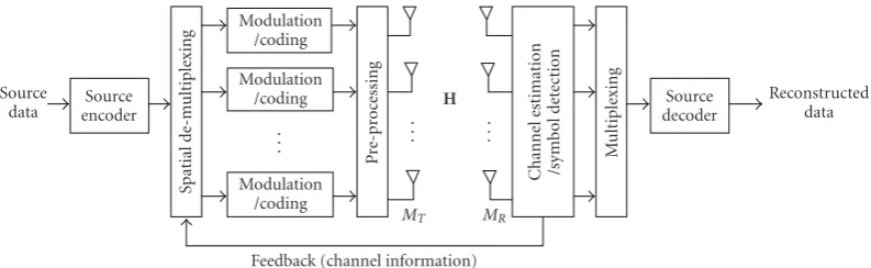
Figure2: Block diagram for the rate control-based closed-loop MIMO system: transmitter and receiver.
From the perspective of the HVS, an optimal power allocation set is determined for delivering the maximal visual
entropy by utilizing Lagrangian relaxation. As a result, the
power level associated with each subband is determined according to the layer of wavelet domain for maximizing visual throughput, which leads to a better visual quality by the numerical and simulation results.
In addition, due to channel variations, transmissions
using different antennas may experience different packet loss
rates using the optimal receiver. In this case, the greater visual quality can be obtained by transmitting the more important data via the best quality channel. Therefore, it is necessary to measure the amount of visual information for each bitstream and then to load the bitstream to a suitable antenna path according to the amount. To quantify the visual importance, visual entropy is introduced. Based on this value, the video data with a more important information is transmitted over a high-quality channel and vice versa. Besides, an adaptive load balance control scheme named equal termination scheduling (ETS) is proposed to give a privilege for high-priority data by avoiding inevitable channel errors over an error-prone channel.
2. SYSTEM OVERVIEW AND ASSUMPTION
2.1. The background area
Generally, the video sequence is coded into a single or multiple bitstreams according to the coding architecture,
which is composed of different codewords including different
degrees of importance. It is quite noticeable that each
codeword contains different visual information so that the
bitstream with different importance can be treated differently
for provisioning higher quality services. In other words, the loss of important data may result in a severe degradation of the decoded video quality. In contrast, the loss of less important data may be tolerable. Therefore, it is necessary to provide better protection to important data, which is the basic idea of unequal error protection (UEP).
Essentially, the UEP method implicates the distribution of errors in order that more important data can experience fewer bit errors without demanding extra resource con-sumption. It has been widely demonstrated that the UEP is
an efficient method in delivering error sensitive video over
error-prone wireless channels [20]. Common approaches
for the UEP are based on forward error correction (FEC)
[21] or modulation scheme, such as hierarchical quadrature
amplitude modulation (QAM) [22]. In [23], a UEP scheme
based on subcarrier allocations in a multicarrier system is also proposed.
In this work, we propose the new UEP technique based on the HVS using the unequal power allocation
and exploit the difference in visual importance of each bit
stream by means of visual entropy using unequal power allocation among multiple antennas. To achieve this main goal, a wavelet-based video coding is used to encode the
video sequence into multiple bitstreams with different visual
contents. For example, in the two-layer video, the base layer with a high weight carries more important visual information as an independently decodable expression with acceptable quality, but the enhancement layer with a low weight carries additional detailed visual information for quality improvement. In addition, the video coder based on the wavelet transform has the desirable property of generating naturally-layered bitstreams, which are composed of low- and high-frequency components. Therefore, the UEP provides stronger protection to the layer, which contains the important visual information.
2.2. At the transmitter side
Figure 2 depicts the block diagram of the MIMO system
withMT andMR antennas at the transmitter and receiver,
respectively. In addition, we assume spatially multiplexing
transmission in whichMTindependent data streams are sent
from each transmit antenna.
Using a progressive wavelet video encoder, for example, set partitioning in hierarchical trees (SPIHT) or embedded block coding with optimized truncation (EBCOT), each layer
can be constructed by scanning wavelet coefficients [24,25].
In this case, each coefficient has a different visual importance
according to the associated spatial and frequency weight. After obtaining the sum of the visual weights for each layer, the value can be included in the header. In terms of the weighted value, it is assumed that the communication system can recognize the importance of each layer.
shown in Figure 2. These layers are subsequently coded, modulated separately, and then transmitted simultaneously on the same frequency. The coding, modulation, and transmit power of each layer are subject to the capacity maximization according the feedback information and the visual information which each layer contains, as depicted inFigure 2. In this paper, the optimization for the maximal capacity experienced over the wireless channel is obtained by using the Shannon capacity. Since the Shannon capacity is a
theoretical upper bound afforded by using communication
techniques, such as the automatic repeat-request (ARQ), forward error correction (FEC), and modulation schemes, it is assumed that the proposed system employs the best ARQ, FEC, and modulation schemes. We assume that a combination of coding and modulation at each antenna is
the same. The only difference is the level of allocated power
at each transmit antenna. If any power is not allocated to the
kth antenna, thekth antenna is not used for transmission.
The power allocation under the total transmit power constraint is one of the roles in the preprocessing stage. It divides the streams into nonoverlapping blocks. The power optimization algorithm then runs on each of these blocks independently with respect to the amount of the visual information. The detail in the optimization procedure will be discussed later. Thus, an optimal power level is allocated to each block by taking into account the visual weight for transmitting data as much as possible from the visual quality point of view.
2.3. The channel model
For numerical analysis, let pkbe the allocated power to the
kth transmit antenna. The signal vector to be sent from
the transmitter is expressed as x = [x1,. . .,xMT]
T
, with
E[xxH]=diag(p
1,p2,. . .,pMT) subject to
MT
i pi=P, where
Pis the total transmit power. The channel response between
the transmitter and the receiver is represented by anMR×MT
MIMO channel matrix as
H= ⎛ ⎜ ⎜ ⎝
h11 · · · h1MT
..
. . .. ...
hMR1 · · · hMRMT
⎞ ⎟ ⎟
⎠, (1)
where hmn (1 ≤ m ≤ MR, 1 ≤ n ≤ MT) is modeled
as a complex Gaussian variable with zero-mean and unit
variance representing the channel response between thenth
transmit antenna and the mth receive antenna. A spatially
uncorrelated channel model is assumed to be used in this paper.
Accordingly, theMR×1 received signal vector is then
y=Hx+n, (2)
where n denotes the MR ×1 independent and identically
distributed zero-mean circularly symmetric complex gaus-sian (ZMCSCG) noise vector with the covariance matrix
E[nnH] = N
oIMR [26–28]. The received signal vector,y, is
then sent to the linear receiver.
2.4. At the receiver side
At the receiver, we assume that the channel is perfectly estimated for the closed-loop MIMO system. Here, three alternative receiver schemes are considered: singular value decomposition (SVD) detection, zero-forcing (ZF) detec-tion, and minimum mean square error (MMSE) detection
[29]. For ease of analysis, it is assumed that the most
powerful channel estimation technique is used. Based on the information at the receiver, the estimated channel value needed to determine the allocated power is then feedback to adjust the corresponding transmission parameters as
mentioned before. Authors in [14] showed that a delay in
feeding the channel status information(CSI) back to the transmitter causes severe degradation in the performance
of SVD systems, and the effect from this was quantified in
[15]. Since this effect is beyond the scope in this paper, it is
assumed that there is neither delay nor error in the feedback channel.
The channel is modeled as a complex Gaussian random variable with zero-mean and unity variance, which is also assumed to be flat fading and quasistatic so that the channel remains constant over the transmission during the execution for the power allocation after the feedback information. It is also assumed to use the optimal channel realization technique for ease of analysis.
After detecting the symbol and deciding the bits at each antenna, the raw data bitstream is then passed to the
multiplexing block. The block converts theseMRbitstreams
into serial streams corresponding to the number of transmit antennas. Finally, the multiplexer combines those streams into a single received bitstream.
2.5. The definition of visual entropy
To measure the visual importance of each layer at the preprocessing stage, it is necessary to decide the cross-layer optimization constraint or criterion. Here, a normalized weight will be adopted as the criterion to quantify the visual
importance of each layer. In [16, 17], we defined “visual
entropy” as the expected number of bits required to represent image information mapped over human visual coordinates.
The visual entropy in [17] is written as
Hdw a[m]
=wmtHd a[m]
=wtm log2σm+ log2
2e2, (3)
where m is the index of wavelet coefficients, a[m] is a
random variable of coefficient with the index m,Hd(a[m])
is the entropy of a[m], wt
m is the visual weight, and σm
is the variance when a[m] has a Laplacian distribution.
Since Hd(a[m]) is the minimum number of bits needed
to represent a[m], the visual entropy can be expressed as
a weighted version ofHd(a[m]) associated with the visual
weightwt
m.
The visual weightwt
mis characterized by using two visual
components: one for the spatial domainws
m, and the other
for the frequency domainwmf as shown inFigure 3.
According to the wavelet decomposition inFigure 3(a),
The low frequency coefficient
The high frequency coefficient
(a) (b) (c) (d)
Figure3: (a) Wavelet decomposition, (b) the weight of the spatial domain, (c) the weight of the frequency domain, and (d) the total weight wavelet domain. The brightness in the figures represents the level of visual importance.
and3(d), respectively. When spatial visual information such
as a region of interest, an object or objects, the nonuniform sampling process of the human eye can be utilized to obtain
ws
m over the spatial domain. In addition, the human visual
sensitivity can be characterized by wmf over the frequency
domain by measuring the contrast sensitivity of the human
eye [30]. Based on this measurement, the total weight over
the two domains can be obtained bywt
m = w
f
m·wms. In the
layered video coding based on the frequency band division without the use of foveation, the weight of each layer
becomes wt
m = w
f
m. In the region-based, object-based, or
foveation-based video coding without the use of the layered
structure, the weight becomeswt
m=wms. In the hybrid video
coding based on an object-based layered mechanism, the weight over the spatial and frequency domains needs to be
taken into account. In this case,wt
m = w
f
m·wms The details
aboutwmf andwsmare discussed in [17].
Since the entropyH(a[m]) is a constant value, the sum
of visual entropy forMcoefficients yields
M−1
m=0
Hw a[m]=M·H a[m]
M−1
m=0 wtm
=M·H a[m]·wt=C w,
(4)
whereCwis the sum of the delivered visual entropies for each
coefficients. The details are described in [17].
Since the HVS is insensitive for distortions in the fast-moving region to a considerable extent, some considerations can be applied to the visual weight for an“I-frame” or a “P-frame,” respectively, according to the temporal activity of video, which is computed as the mean value of motion
vectors in the frame. Authors in [31] proposed a quality
metric for video quality assessment using the amplitude of motion vectors and evaluated it in accordance with a sub-jective quality assessment method such as double-stimulus continuous quality scale (DSCQS) and single-stimulus
con-tinuous quality evaluation (SSCQE) [32]. Therefore, it is
necessary to consider the temporal extent using motion vectors for obtaining visual entropy for the video sequence.
The temporal activity of theith frameTAiis, then, defined
as
TAi=mvx,i(x,y)+mvy,i(x,y), 1≤x≤W, 1≤y≤H,
(5)
where |mvx,i(x,y)| and |mvy,i(x,y)| represent the mean
values of the horizontal and vertical components of the
motion vector at the spatial domain (x,y) in theith frame,
andWandHare the width and height of the video sequence,
respectively.
Reflecting the temporal activity, the visual weightwm can
be redefined as
wm = wm
c1+ max TAi,c2 2
/c3
, (6)
wherec1,c2, andc3are constants determined by experiments
and are used by “2.5,” “5,” and “30” in [31]. For brevity, it is
assumed thatwm is expressed bywmthrough this paper.
2.6. The unequal power allocation with multiple antennas
The UEP can be implemented by utilizing the differences
in the channel quality among the multiple antennas. The general UEP method has taken only the dynamics of the channel situation into account, and the UEP based on the water-filling method has been known as an optimal solution
for maximum channel throughput [8, 9]. In contrast, in
this paper, the amount of visual information is used as the optimal value of the object function for a given power constraint.
In the scheme, the video sequence is decoded into several bitstreams using a layered wavelet video. Each layer includes
a different degree of importance which is quantified by
means of visual entropy. An unequal power allocation (UPA) algorithm may be then performed in real-time. However, in general, intensive computation may be required to obtain an optimal solution. To reduce the computational complexity, we derive a closed numerical form of the optimal power for the power allocation method.
The proposed UPA technique consists of two steps: antenna selection based on the channel gain, and optimal
power allocation according to the visual weight inFigure 3.
The multiple antennas can be classified and ordered based on the metric of the channel gain. To perform this antenna selection at any instantaneous channel realization, we mea-sure the channel for each antenna using a channel estimation. More specifically, the antenna with the best channel gain is labeled as the 4th antenna, and the antenna with the second
Step 1) Different priority data are stacked in a different priority downlink queue.
Step 2) All packets are virtually arranged by the DL scheduler as if they are stacked in a single queue.
Step 3) Arranged packets are divided by the divisor (the number of antennas). Then, the scheduler makes an index for each packet.
Step 4) The DL scheduler makes a plan for transmitting packets: how much packets are taken out from each queue at a certain time slot.
Step 5) The DL scheduler transmits the packet taken out from the queue in accordance with the table plan in step 4. 1 2 1 2 1 2
A B C D E F
Slot 1 Slot 2 Time
Draw
2 packets fromQ1 0 packet fromQ2 1 packet fromQ3
Draw
1 packet fromQ1 1 packet fromQ2 1 packet fromQ3
A B E C D F
DL scheduler
F E
D
A B C
Q3
Q2
Q1
Lo
w
Hi
gh
Queue
Queue
Queue
DL scheduler
Q1 Q2 Q3
2 0 1
1 1 1
Time slot 1 Time slot 2
Hi
gh
Pr
io
ri
ty
Lo
w Q3
Q2
Q1
F E
D
A B C
Figure4: A conceptual example of the ETS algorithm.
After performing the antenna selection and assignment
for different streams, a power is then allocated to each
antenna according to the visual weight of the associated video layer. Hence, more power can be allocated to more important layer, resulting in a further increase in the overall visual throughput. Therefore, the visually important data will experience less packet errors, and vice versa.
2.7. The adaptive load control using the ETS algorithm
It is assumed that each layer consists of the packets, and the
number of packets in each layer may be different from those
of the others. In the downlink scheduler, each layer is stacked into the corresponding queue as the unit of the packet according to its priority. Since the priority is determined based on the visual importance carried in the packet so that the packet classification is accomplished through queues in the scheduler.
The procedure of the ETS algorithm is described in detail as follows.
(1) Step 1: based on the visual weight, which each packet contains, the transmission priority is determined so that it
can be stacked in the corresponding queue. InFigure 4, the
queue of Q1 has the highest priority, which contains three
packets notatedA,B, andC. the priority is decreased in the
order ofQ1,Q2, andQ3.
(2) Step 2: all the packets in the queues are virtually arranged by the scheduler as if they are stacked in a single
queue as shown inFigure 4.
(3) Step 3: the arranged packets are divided by the divisor which is the number of transmit antennas. The scheduler then makes an index for each packet. It is assumed that three channels are available so that the arranged packets are divided into three subgroups.
(4) Step 4: the scheduler makes a plan for transmitting the packets: how many packets are drawn in each queue at each time slot. For example, the total number of packets is 6 over the three available antennas so that two-time slots
are required to transmit all the packets. InQ1, two packets
are transmitted at the first time slot and one packet is
transmitted in the second time slot. In case ofQ2, no packet
is transmitted in the first time slot, and the remaining packet is transmitted in the second time slot.
(5) Step 5: the scheduler transmits the packet from the queue in accordance with the table obtained in step 4.
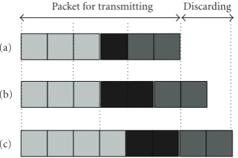
Packet for transmitting Discarding
(a)
(b)
(c)
Figure5: Tail packets are discarded regardless of their weights in the ETS algorithm.
packets if the channel capacity is not enough to transmit all the packets. The issue is how to deal with remaining packets
and the solution, the tail packet discarding, is proposed as
depicted inFigure 5.
For example, Figures 5(a) and 5(b) are the cases of
requiring 3 time slots with 2 antennas, andFigure 5(c) is the
case of requiring 2 time slots with 3 antennas. The remainder occurs when the number of packets is not exactly divided by the divisor. In such a case, the remaining packets are discarded regardless of its visual weight, since the visual weight of the remaining packets are relatively smaller for the previous queueing and virtual arrangement. Thus, utilizing the ETS algorithm, the throughput of visually important data can be maintained while delivering the packets in the order of arrival at the scheduler. The policy of tail packet dropping
contributes an efficient use of resources for delay sensitive
but loss tolerant video traffic.
3. OPTIMAL POWER CONTROL USING LAGRANGIAN RELAXATION
In this section, a numerical analysis for cross-layer optimiza-tion is described to maximize the amount of the transmitted
data over the MIMO system. In particular, we make an effort
to transmit the visual information as much as possible for a given channel capacity. Thus, in the optimization problem, the source rate is expressed by means of visual entropy, and the channel capacity is calculated by Shannon theorem.
To maximize visual entropy, an optimization problem can be formulated as follows:
(A) max
M
m=1
Hw a[m],
subject to
M
m=1
H a[m]≤C,
(7)
whereH(X) is the entropy of a random variableX,Hw(X)
is the visual entropy of X,m is the index of coefficients,
andCis the channel capacity. This objective function for the
optimization will be more specified according to the type of the receiver as follows.
Precoder V
Channel H
Decoder UH
x y
x y
n
Figure6: Utilizing precoder and decoder via decomposition ofH
when the channel is known to both transmitter and receiver.
3.1. SVD (singular value decomposition) receiver
In [29], the eigen-mode spatial multiplexing method is
studied by performing singular value decomposition (SVD) on the channel response matrix. Through precoding at the transmitter and decoding at the receiver, the channel matrix is converted into a matrix as
Σ=UHHV
= ⎛ ⎜ ⎜ ⎜ ⎜ ⎜ ⎝
λ1 0 0
. ..
0 λr
0 . . . 0 M
T−r
× MR−r
⎞ ⎟ ⎟ ⎟ ⎟ ⎟ ⎠,
(8)
wherer ≤min{MT,MR}is the rank ofH, andλ1,λ2,. . .,λr
are the eigenvalues of the channel matrixHHH. TermsUH
andVare theMR×MRandMT×MTunitary matrices that are
used as the decoding and precoding matrices, respectively.
Therefore, (2) becomes
y=Hx+n
=UΣVHx+n. (9)
By multiplyingVandUHtoxandy, (9) is transformed
into
UHy=y
=UHHVx+UHn
=UHHVx+n
=UHUΣVHVx+n =Σx+n.
(10)
Figure 6shows the schematic channel model ofeigen-mode transmissionwhen the channel is known to the transmitter and receiver.
Equation (10) shows thatHcan be explicitly decomposed
into r parallel single input single output (SISO) channels
satisfying
yk=
λkxk+n (11)
when the transmitter knows the channel matrix.
Since UH is a unitary matrix, UHn has the same
covariance asn, and thus the postprocessing SNR for thekth
data stream is
SNRk= pk
Noλk
, (12)
where pk = E{|xk|2},
MT
k pk ≤ P,λk is 0 if k > r. pk
reflects the transmit energy in theith subchannel and satisfies
MT
From (12), it is clear that the received SNR of each data stream is proportional to its transmit power. Furthermore, since the transmission rate is continuous, the optimum strategy for power allocation is simply based on the
water-filling theory [1].
To obtain the optimum power value using SVD, (7) can
be transformed to a new problem by (12) as follows:
(B1) max
pk
r
k=1 wtk·log2
1 + pk
Noλk
,
subject to
r
k=1
pk≤P, pk≥0
(13)
wherePis a total transmit power with respect to all transmit
antennas, and wtk is the value of the visual weight in the
transmitted layer corresponding to the assignedkth transmit
antenna. The solution in (13) is an optimal power set,
{p1,p2,. . .,pMT}. Because (13) is a convex problem, we can
apply to the Karush-Kuhn-Tucker (KKT) condition with
respect to pk to obtain an optimal power set which is a
globally optimum solution. Using a Lagrangian relaxation,
L(pk,ν)= r
k=1 wtk·log2
1 + pk
Noλk
+ν P− r
k=1 pk
, (14)
whereνis a nonnegative Lagrangian multiplier. Taking the
derivatives with respect to pk and ν can be obtained as
follows:
∂L ∂pk =w
t k·
λk/No
1 +pkλk/No
ln 2−ν≤0, (15)
pk·∂L
∂pk =
0, (16) ν P− r
k=1 pk
=0. (17)
From (15) and (16), if powerpk is allocated to thekth data
stream (i.e.,pk≥0), the complementary slackness condition
is then satisfied as follows:
wtk·
λk/No
1 +pkλk/No
ln 2=ν. (18)
In addition, the optimal values ofpkand its multiplierνare
given by
pk=
wt k
νln 2−
No
λk. (19)
Substituting (17) with (19),
1
νln 2 =
P+No
r k=1 1/λk
r
k=1wtk
. (20)
Substituting (21) with (20),
pk=
wt k
r k=1wtk
P+No r
k=1 1
λk
−No
λk. (21)
3.2. MMSE (minimum mean square error) receiver
The MMSE matrix filter for extracting the received signal
into thekth component transmitted stream is given by
GMMSE=hHk
NoIMR+
MT
i /=k
pihihHi
−1
, (22)
wherehkis thekth column ofH, that is,MR×1 vector. Thus,
the SINR for thekth data stream can be expressed as
SINRk=pkhHk
NoIMR+
MT
i /=k
pihihHi
−1
hk=pkgk, (23)
wheregk=hHk(NoIMR+
MT
i /=kpihihHi )
−1 hk.
To obtain the optimum power value using the MMSE
receiver, (7) can be transformed to a new problem using (23)
as follows:
(B3) max
pk
MT
k=1
wtk·log2 1 +pkgk
,
subject to
MT
k=1
pk≤P, pk≥0.
(24)
Equation (24) is also a convex problem, we can apply to the
KKT condition with respect topkto obtain an optimal power
set. By using a Lagrangian relaxation,
L pk,ν
=
MT
k=1
wtk·log2 1 +pkgk
+ν P− MT
k=1 pk
, (25)
whereνis a nonnegative Lagrangian multiplier. Taking the
derivatives with respect topkandν, respectively, then
∂L ∂pk =w
t k·
gk
1 +pkgk
ln 2 −ν≤0, (26)
pk·∂L
∂pk =
0, (27) ν P− MT
k=1 pk
=0. (28)
Using (26) and (27), the complementary slackness
condition is given by
wt k·
gk
1 +p∗kgk
ln 2 =ν. (29)
The optimal power is obtained by
p∗k =
1
gk
−1 +w
t k·gk
νln 2
. (30)
Using (28) and (30),
1
νln 2 =
P+MT
k=1 1/gk
MT
k=1wtk·gk
. (31)
Using (30) and (31),
pk=
1
gk
−1 + w
t k·gk
MT
k=1wtk·gk
P+
MT
k=1 1
gk
Table1: Visual weight for each layer.
Layer 1 Layer 2 Layer 3 Layer 4
Visual weight (I-frame) 0.09236 0.12258 0.17951 0.45107
Visual weight (P-frame) 0.12568 0.16728 0.24783 0.45920
3.3. ZF (zero forcing) receiver
The zero forcing (ZF) matrix filter for extracting the received signal into its component transmitted streams is given by
GZF= HHH −1
HH, (33)
whereGZFis anMT×MRpseudo-inverse matrix that simply
inverts the channel. The output of the ZF receiver is given by
GZFy=x+ HHH −1
HHn. (34)
Thus, the postprocessing SNR for thekth data stream in [26–
28] can be expressed as
SNRk= pk
No
HHH−1 k,k
. (35)
To obtain the optimum power value using the ZF
receiver, (7) can be transformed to a new problem using (35)
as follows:
(B2) max
pk
MT
k=1 wt
k·log2
1 + pk
No[HHH]−k,1k
,
subject to
MT
k=1
pk≤P, pk≥0.
(36)
The solution of the optimization problem in (36) is
an optimal power set, {p1,p2,. . .,pMT} for each antenna.
Because (36) is a convex problem, we apply the KKT
condition with respect topkto obtain an optimal power set
which is a globally optimum solution. By using a Lagrangian relaxation,
L pk,ν
=
MT
k=1 wt
k·log2
1 + pk
No[HHH]−k,1k
+ν
P−
MT
k=1 pk
,
(37)
whereνis a nonnegative Lagrangian multiplier. Taking the
derivatives with respect to pkandν, respectively, yields the
KKT conditions as follows:
∂L ∂pk =w
t k·
1/No
HHH−1 k,k
1 +pk/No
HHH−1 k,k
ln 2−ν≤0, (38)
pk·∂L
∂pk =
0, (39)
ν
P−
MT
k=1 pk
=0. (40)
From (38) and (39), ifpkis allocated to thekth data stream
(i.e.,pk≥0), the complementary slackness condition is then
satisfied as follows:
wt k·
1/No
HHH−1 k,k
1 +p∗k/No
HHH−1 k,k
ln 2 =ν. (41)
The optimal value ofp∗k is given by
p∗k = wtk
νln 2−No
HHH−k,1k. (42)
Substituting (40) with (42),
1
νln 2 =
P+No
MT
k=1
HHH−1 k,k
MT
k=1wtk
. (43)
Substituting (44) with (43), the optimal power can be
obtained by
p∗k =
wt k
MT
k=1wtk
P+No MT
k=1
HHH−1 k,k
−No
HHH−1 k,k. (44)
In short, the optimal power sets for maximizing visual entropy for the cases of SVD, MMSE, and ZF receivers are
(21), (32), and (44), respectively.
4. NUMERICAL RESULTS
In the simulation, the three different types of linear receivers
are adopted for performance comparison. First of all, the major parameters used for the simulation are SNR: 0 dB, the number of transmit antennas: 4, the number of receive antennas: 4, and the total transmit power: 1. The “Lena”
(frame size −256 by 256) is used to apply the proposed
algorithm to the I-frame analysis, and the “Stefan” (frame size−352 by 240, frame rate−15 frame/second) is used to apply it to the P-frame analysis. The total transmit power is normalized to analyze with ease.
We made the encoded data from the “Lena” image
using the modified SPIHT in [33]. First, after extracting the
coefficients from the first sorting and refinement pass, the
visual weight of these data is obtained. Similarly, the visual weights are calculated for the next three data extracted from the next passes, and four layers were loaded to the transmit antenna according to the visual weight.
In addition, the visual weight wtk for each layer or
bitstream in (4) is used for the simulation as listed inTable 1,
and the amount of visual information can be different
according to the visual weight in Table 1 ((a) and (b)
represent the visual weight for the “Lena” and “Stefan,” resp.)
(a) (b) (c) (d)
Figure7: The reconstructed images without the 1st, 2nd, 3rd, and 4th layer data, from (a) to (d), respectively.
0 0.5 1 1.5 2 2.5 3 3.5 4
Su
m
o
f
capacit
y
(bits/Hz)
SVD MMSE ZF
Receiver type Proposed
Water-filling Equal
(a)
0 0.2 0.4 0.6 0.8 1 1.2 1.4
Su
m
o
f
visual
ent
ro
p
y
(bits/Hz)
SVD MMSE ZF
Receiver type Proposed
Water-filling Equal
(b)
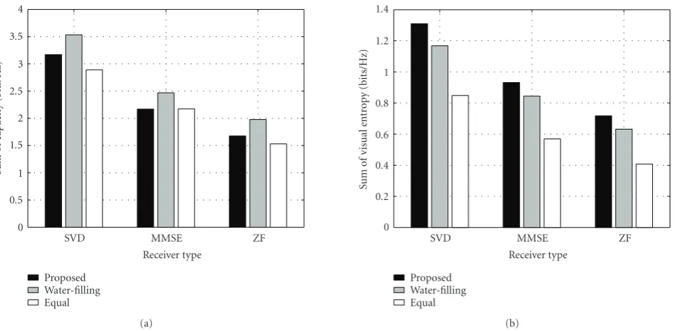
Figure8: The sum capacity versus the sum of visual entropy according to the receiver configuration.
Figure 7represents the images reconstructed without the 1st, 2nd, 3rd, and 4th layer data, respectively, assuming that the higher number layer has more important data, which will load to an antenna with a higher number. In other words, each subfigure represents the reconstructed data without
information as much as the visual weight,wt1,wt2,wt3, andwt4,
respectively. Whereas the image inFigure 7(a) without the
1st information has a relatively small degradation for quality,
the image inFigure 7(d)has the poorest quality among all the
images due to the loss of the information in the 4th layer, and this shows that the 4th layer has the most visually important data. The quantity of this information can be calculated by means of the visual weight.
A common channel matrix ofH, the ZMCSCG channel
is used, and the uncorrelated channel is only considered in the numerical analysis.
Figure 8 shows the sum rate of the capacity and the total visual entropy according to the linear receiver. The
sum rate is measured by Shannon capacity theorem [26] for
the unequal power allocation scheme and by the conven-tional water-filling scheme. As mentioned, the general UEP methods have used only the channel quality metric to apply the water-filling scheme, but the proposed method achieves a maximal visual throughput via visual entropy. Although an absolute maximal volume of the transmitted data for the proposed method can be lower than that of the water-filling scheme, the proposed system can obtain greater visual information compared to the water-filling scheme.
In addition, it can be seen inFigure 8that the channel
0 0.1 0.2 0.3 0.4 0.5 0.6 0.7 0.8 0.9
Allocat ed p o w er le ve l
1 2 3 4
Layer Proposed Water-filling Equal
Allocated power: SVD receiver
(a)
0 0.5 1 1.5 2 2.5 3 T ransmitt ed b its (bits/Hz)
1 2 3 4
Layer Proposed Water-filling Equal
Transmitted bits: SVD receiver
(b)
0 0.2 0.4 0.6 0.8 1 1.2 1.4
V isual ent rop y (bits/Hz)
1 2 3 4
Layer Proposed Water-filling Equal
Visual entropy: SVD receiver
(c)
0 0.1 0.2 0.3 0.4 0.5 0.6 0.7 0.8 0.9 1 Allocat ed p o w er le ve l
1 2 3 4
Layer Proposed Water-filling Equal
Allocated power: MMSE receiver
(d)
0 0.2 0.4 0.6 0.8 1 1.2 1.4 1.6 1.8 2 T ransmitt ed b its (bits/Hz)
1 2 3 4
Layer Proposed Water-filling Equal
Transmitted bits: MMSE receiver
(e)
0 0.1 0.2 0.3 0.4 0.5 0.6 0.7 0.8 0.9 1 V isual ent rop y (bits/Hz)
1 2 3 4
Layer Proposed Water-filling Equal
Visual entropy: MMSE receiver
(f)
0 0.1 0.2 0.3 0.4 0.5 0.6 0.7 0.8 0.9 1 Allocat ed p o w er le ve l
1 2 3 4
Layer Proposed Water-filling Equal
Allocated power: ZF receiver
(g)
0 0.2 0.4 0.6 0.8 1 1.2 1.4 1.6
T ransmitt ed b its (bits/Hz)
1 2 3 4
Layer Proposed Water-filling Equal
Transmitted bits: ZF receiver
(h)
0 0.1 0.2 0.3 0.4 0.5 0.6 0.7
V isual ent rop y (bits/Hz)
1 2 3 4
Layer Proposed Water-filling Equal
Visual entropy: ZF receiver
(i)
(a) (b) (c)
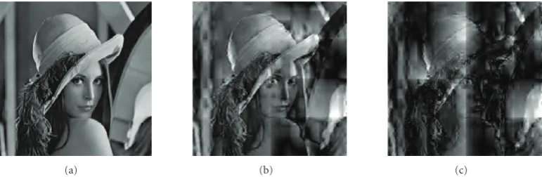
Figure10: “Lena” images using (a) the proposed, (b) the water-filling, and (c) the equal power methods.
(a) (b) (c)
Figure11: The 2nd frame for “Stefan” using (a) the proposed, (b) the water-filling, and (c) the equal power methods.
given channel condition, but the visual QoS is significantly enhanced from the users point of view.
Figures 9(a), 9(d), and 9(g) show optimal power sets
using (19), (42), and (30), which are the solutions of (13),
(36), and (24), respectively. In the ETS scheme, the optimal
set of power is determined according to the visual weight carried in each packet. Although the same amount of data
is delivered over each band, each bitstream has a different
visual information. Since the 4th layer has the most sensitive visual information in terms of the HVS, it can be seen that the highest power is allocated to the 4th SISO channel. The power patterns for the rest of the layers are relatively smaller compared to other power allocation algorithms.
The findings show that an increase in the allocated power of the 4th layer results in an improvement in throughput
as shown inFigure 9. Since the visual weight of the layer is
the greatest compared to the other layers, it is expected that much higher visual entropy can be delivered by using the unequal power allocation according to the visual importance.
Figures 9(b), 9(e), and 9(h) show the number of
transmitted bits using (13), (36), and (24), respectively,
where the value ofwkbis assumed to “one.” Under the given
channel environment, the UPA based on the water-filling can transmit the more number of bits over the antenna arrays. The proposed scheme allocates a higher power for the 4th layer, it can be seen that the throughput of the layer is relatively lower than that of the water-filling case.
Figures 9(c), 9(f), and 9(i) show the values of visual
entropy using (13), (36), and (24), respectively. In the view
of visual entropy, it can be found that the proposed method demonstrates the best performance. Moreover, additional visual entropy gain can be achieved because a greater power is allocated to the bitstream of the 4th band. The similar tendencies can be founded regardless of the receiver type.
Even if the number of the total transmit bits for the proposed method is lower than that of the water-filling scheme, the throughput of visual data can be significantly increased due to the UPA for each layer in the order of visual entropy.
Figure 10 shows the reconstructed images using the proposed, water-filling, and equal power methods when the SVD transmission is employed as the linear receiver. Due to the less throughput of visual entropy in the other schemes, the visual quality is much degraded compared to the proposed scheme. In case of the proposed method, even though it does not receive any 1st or 2nd information, the received image can have the best quality by protecting the most important data. It can be seen that these results are,
therefore, consistent to the numerical results in Figures 8
and9.
Figure 11 shows the reconstructed frames for “Stefan” using the proposed, water-filling, and equal power methods when the SVD transmission is employed as the linear receiver. It is assumed that the previous I-frame (i.e., the 1st frame) is transmitted with an error-free channel, and data with respect to only the motion vector is loaded to the MIMO antennas. These results are consistent to the previous results
5. CONCLUSION
In this paper, we considered the realization of UEP in the MIMO system using the channel feedback, in which data can be transmitted simultaneously through multiple antennas.
We proposed an effective way to improve the error resilience
of compressed video based on a cross-layer approach. Due
to two-dimensional characteristics of video, that is, different
portions of video data have different importance, video data
can be divided in the metric of visual entropy. In this work, we employ an image quality metric and visual entropy to quantify the image quality. Due to channel variations and the
amount of the allocated power, transmissions on different
antennas may experience different packet loss rates. Thus,
to achieve the different error distribution according to data
with different visual weight, data with higher priority is
transmitted in order to achieve higher channel gain for lower loss and error rate, and data with lower priority is on the remaining channel. Meanwhile, an adaptive load balance control scheme is proposed to give a privilege for high-priority data by passing transmission errors to data with lower priority for avoiding inevitable channel errors over an error-prone channel. The simulation results demonstrate that the proposed adaptive transmission scheme achieves significantly better performance than existing conventional systems.
ACKNOWLEDGMENTS
This work was supported by the Korea Science and Engine-ering Foundation Grant funded by the Korea government (MOST) (no. R01-2007-000-11708-0), and Seoul Research & Business Development Program (11136M0212351).
REFERENCES
[1] I. E. Telatar, “Capacity of multi-antenna Gaussian channels,”
European Transactions on Telecommunications, vol. 10, no. 6, pp. 585–595, 1999.
[2] G. J. Foschini and M. J. Gans, “On limits of wireless com-munications in a fading environment when using multiple antennas,”Wireless Personal Communications, vol. 6, no. 3, pp. 311–335, 1998.
[3] H. Zheng, “Optimizing wireless multimedia transmissions through cross layer design,” in Proceedings of the IEEE International Conference on Multimedia and Expo (ICME ’03), vol. 1, pp. 185–188, Baltimore, Md, USA, July 2003.
[4] A. K. Katsaggelos, Y. Eisenberg, F. Zhai, R. Berry, and T. N. Pappas, “Advances in efficient resource allocation for packet-based real-time video transmission,”Proceedings of the IEEE, vol. 93, no. 1, pp. 135–146, 2005.
[5] E. Setton, T. Yoo, X. Zhu, A. Goldsmith, and B. Girod, “Cross-layer design of ad hoc networks for real-time video streaming,”
IEEE Wireless Communications, vol. 12, no. 4, pp. 59–64, 2005. [6] H. Jiang, W. Zhuang, and X. Shen, “Cross-layer design for resource allocation in 3G wireless networks and beyond,”IEEE Communications Magazine, vol. 43, no. 12, pp. 120–126, 2005. [7] N. Conci, G. B. Scorza, and C. Sacchi, “A cross-layer approach for efficient MPEG-4 video streaming using multicarrier spread-spectrum transmission and unequal error protection,” inProceedings of the IEEE International Conference on Image
Processing (ICIP ’05), vol. 1, pp. 201–204, Genova, Italy, September 2005.
[8] M. F. Sabir, R. W. Heath Jr., and A. C. Bovik, “Unequal power allocation for JPEG transmission over MIMO systems,” in
Proceedings of the 39th Asilomar Conference on Signals, Systems and Computers, pp. 1608–1612, Pacific Grove, Calif, USA, October-November 2005.
[9] M. F. Sabir, R. W. Heath Jr., and A. C. Bovik, “An unequal error protection scheme for multiple input multiple output systems,” in Proceedings of the 36th Asilomar Conference on Signals Systems and Computers, vol. 1, pp. 575–579, Pacific Grove, Calif, USA, November 2002.
[10] M. Tesanovic, D. Bull, A. Doufexi, and A. Nix, “Analysis of IEEE 802.11n-like transmission techniques with and without prior CSI for video applications,” inProceedings of the IEEE International Conference on Image Processing (ICIP ’07), vol. 6, pp. 493–496, San Antonio, Tex, USA, September 2007. [11] N. Gogate, D.-M. Chung, S. S. Panwar, and Y. Wang,
“Supporting image and video applications in a multihop radio environment using path diversity and multiple description coding,”IEEE Transactions on Circuits and Systems for Video Technology, vol. 12, no. 9, pp. 777–792, 2002.
[12] S. Lin, A. Stefanov, and Y. Wang, “Joint source and space-time block coding for MIMO video communications,” in
Proceedings of the 60th IEEE Vehicular Technology Conference (VTC ’04), vol. 4, pp. 2508–2512, Los Angeles, Calif, USA, September 2004.
[13] M. Tesanovic, D. R. Bull, A. Doufexi, and A. R. Nix, “H.264-based multiple description coding for robust video transmission over MIMO systems,”Electronics Letters, vol. 42, no. 18, pp. 1028–1030, 2006.
[14] G. Lebrun, J. Gao, and M. Faulkner, “MIMO transmission over a time-varying channel using SVD,”IEEE Transactions on Wireless Communications, vol. 4, no. 2, pp. 757–764, 2005. [15] M. Tesanovic, D. R. Bull, A. Doufexi, V. Sgardoni, and A. R.
Nix, “Impact of CSI latency on video quality in MIMO systems employing singular value decomposition,”Electronics Letters, vol. 43, no. 18, pp. 972–973, 2007.
[16] H. Lee and S. Lee, “Visual data rate gain for wavelet foveated image coding,” inProceedings of the IEEE International Confer-ence on Image Processing (ICIP ’05), vol. 3, pp. 41–44, Genova, Italy, September 2005.
[17] H. Lee and S. Lee, “Visual entropy gain for wavelet image coding,”IEEE Signal Processing Letters, vol. 13, no. 9, pp. 553– 556, 2006.
[18] S. Lee, M. S. Pattichis, and A. C. Bovik, “Foveated video compression with optimal rate control,”IEEE Transactions on Image Processing, vol. 10, no. 7, pp. 977–992, 2001.
[19] S. Lee, M. S. Pattichis, and A. C. Bovik, “Foveated video quality assessment,”IEEE Transactions on Multimedia, vol. 4, no. 1, pp. 129–132, 2002.
[20] L. Hanzo and J. Streit, “Adaptive low-rate wireless video phone schemes,”IEEE Transactions on Circuits and Systems for Video Technology, vol. 5, no. 4, pp. 305–318, 1995.
[21] D. G. Daut and J. W. Modestino, “Two-dimensional DPCM image transmission over fading channels,”IEEE Transactions on Communications, vol. 31, no. 3, pp. 315–328, 1983. [22] ETSI, “Digital video broadcasting (DVB); framing structure,
channel coding and modulation for digital terrestrial televi-sion (DVB-T),” Tech. Rep. ETSI EN 300 744, V1.4.1, European Telecommunication Standard Institute, Sophia Antipolis, France, 2001.
of the 23rd Annual Joint Conference of the IEEE Computer and Communications Societies (INFOCOM ’04), vol. 2, pp. 1200– 1210, Hongkong, March 2004.
[24] A. Said and W. A. Pearlman, “A new, fast, and efficient image codec based on set partitioning in hierarchical trees,”IEEE Transactions on Circuits and Systems for Video Technology, vol. 6, no. 3, pp. 243–250, 1996.
[25] D. S. Taubman and M. W. Marcellin, JPEG2000 Image Compression Fundamental, Standards and Practice, Kluwer Academic Publishers, Dordrecht, The Netherlands, 2002. [26] A. Paulraj, R. Nabir, and D. Gore, Introduction to
Space-Time Wireless Communications, Cambridge University Press, Cambridge, UK, 2003.
[27] D. Tse and P. Viswanath,Fundamentals of Wireless Communi-cation, Cambridge University Press, Cambridge, UK, 2005. [28] A. Goldsmith,Wireless Communications, Cambridge
Univer-sity Press, Cambridge, UK, 2005.
[29] H. Sampath, P. Stoica, and A. Paulraj, “Generalized linear precoder and decoder design for MIMO channels using the weighted MMSE criterion,”IEEE Transactions on Communi-cations, vol. 49, no. 12, pp. 2198–2206, 2001.
[30] J. L. Mannos and D. J. Sakrison, “The effects of a visual fidelity criterion on the encoding of images,”IEEE Transactions on Information Theory, vol. 20, no. 4, pp. 525–536, 1974. [31] F. Yang, S. Wan, Y. Chang, and H. R. Wu, “A novel objective
no-reference metric for digital video quality assessment,”IEEE Signal Processing Letters, vol. 12, no. 10, pp. 685–688, 2005. [32] ITU-T Recommendation BT.500-10, “Methodology for the
subjective assessment of the quality of television pictures,” 2000.