Volume 2007, Article ID 37481,12pages doi:10.1155/2007/37481
Research Article
Quaternionic Lattice Structures for Four-Channel
Paraunitary Filter Banks
Marek Parfieniuk and Alexander Petrovsky
Department of Real-Time Systems, Faculty of Computer Science, Bialystok Technical University, Wiejska 45A street, 15-351 Bialystok, Poland
Received 31 December 2005; Revised 1 October 2006; Accepted 9 October 2006 Recommended by Gerald Schuller
A novel approach to the design and implementation of four-channel paraunitary filter banks is presented. It utilizes hypercomplex number theory, which has not yet been employed in these areas. Namely, quaternion multipliers are presented as alternative pa-raunitary building blocks, which can be regarded as generalizations of Givens (planar) rotations. The corresponding quaternionic lattice structures maintain losslessness regardless of coefficient quantization and can be viewed as extensions of the classic two-band lattice developed by Vaidyanathan and Hoang. Moreover, the proposed approach enables a straightforward expression of the one-regularity conditions. They are stated in terms of the lattice coefficients, and thus can be easily satisfied even in finite-precision arithmetic.
Copyright © 2007 M. Parfieniuk and A. Petrovsky. This is an open access article distributed under the Creative Commons Attribution License, which permits unrestricted use, distribution, and reproduction in any medium, provided the original work is properly cited.
1. INTRODUCTION
Paraunitary filter banks (PUFBs) can be considered the most important among multirate systems [1]. This results from the fact that such filter banks are lossless in addition to guar-anteeing perfect reconstruction. A clear relation between the fullband and subband signal energies greatly simplifies the-oretical considerations, and hence makes PUFBs useful for applications such as image coding.
The paraunitary property means that the basis func-tions related to the subbands of a filter bank are orthogo-nal. However, it is more convenient to work with the anal-ysis polyphase transfer matrix E(z), which is paraunitary if EH(z−1)E(z) = cI
M, wherec is a nonzero constant and
M denotes the number of channels [2]. Thus, instead of constraining the impulse response coefficients, the usual way to obtain a PUFB is to compose its polyphase ma-trix from suitable building blocks. From a different point of view, the matrix is appropriately factorized. In this way, other properties of the filter frequency responses can be si-multaneously imposed, such as linear phase (LP), pairwise-mirror-image (PMI) symmetry, and regularity. The selec-tion and arrangement of factorizaselec-tion components are de-cisive.
Lattice and dyadic-based factorizations of paraunitary polyphase matrices can be distinguished. The first approach utilizes Givens (planar) rotations [2]. They are implemented with the help of a specific structure, whose shape is the reason for using the name “lattice.” The second technique is based on Householder reflections and degree-one building blocks, which are of a different nature [3]. The lattice structures are more frequently used because the structural imposition of the above-mentioned additional properties is easier [4–6].
A serious practical problem with the factorizations for PUFBs is that they lose essential properties in the case of finite-precision implementation. The only exception is the two-band lattice structure reported in [7]. These facts are not widely known because the effects of coefficient quantiza-tion in PUFBs were studied only in [8]. This is undoubtedly a consequence of the growing popularity of lifting factor-izations, which guarantee perfect reconstruction under finite precision [9,10]. However, they lead to biorthogonal systems with a complicated relation between the fullband and sub-band signal energies.
alternative paraunitary building blocks, which can be viewed as generalizations of Givens rotations. The lattice structures based on them maintain losslessness regardless of coefficient quantization [11]. Moreover, the one-regularity conditions can be expressed in terms of the lattice coefficients and thus satisfied even under finite precision [12].
The limitation of the applicability of the technique to the case of four channels is undoubtedly a serious disadvan-tage. However, the proposed solution can be recognized as an extension of the two-band lossless lattice presented in [7]. Moreover, our development can stimulate further researches aimed at its generalization, on the one hand, and practical applications, on the other hand.
The organization of the paper is as follows. InSection 2, the conventional lattice structures for PUFBs are briefly re-viewed to provide the necessary background for further dis-cussion. Losslessness and regularity are approached more closely, and the effect of coefficient quantization on these properties is accentuated. Section 3 introduces a quater-nionic multiplier as an alternative building block for four-channel PUFBs. In Section 4, quaternionic variants of the factorizations fromSection 2are derived, as well as the one-regularity conditions on their coefficients. The advantages of the proposed solution, related to finite-precision implemen-tations, are emphasized. The obtained results are exploited inSection 5, where three representative PUFB design exam-ples are shown. Finally, some concluding remarks are given inSection 6.
Notations 1. Column vectors are denoted by lowercase bold-faced characters, whereas matrices by the uppercase ones. The notationamnrefers to the (m,n) entry of a matrixA.Im andJmdenote them×midentity and reverse identity matri-ces, respectively. The superscriptT stands for transposition. Quantization is indicated withQ(·). Three specific vectors e=[1 0 0 0]T,a=[1 1 0 0]T, ando=[1 1 1 1]Tare helpful. TheL2-norm is considered in our discussion.
2. CONVENTIONAL LATTICE STRUCTURES
2.1. Four-channel general PUFB
The most essential issue in lossless system design is how to obtain anM×Mparaunitary polyphase transfer matrixE(z) of a given McMillan degree [2]. No other properties are re-quired.
At the first successful attempt to solve this problem [13], the factorization
E(z)=RN−1Λ(z)RN−2Λ(z)· · ·R1Λ(z)E0 (1)
was used. It contains the delays
Λ(z)=diagz−1,I
M−1
(2)
and orthogonal matrices: a general one,E0, withM(M−1)/2
degrees of freedom, andRi,i=1,. . .,N−1, constrained to haveM−1 of these. Both kinds of matrices are commonly implemented using Givens (planar) rotations, each of which corresponds to one degree of freedom [2].
z 1
z 1
z 1 4 4 4 4
α0,0
α0,3 α0,1
α0,5 α0,4 α0,2
z 1 z 1
α1,0
α1,1
α1,2
α2,0
α2,1
α2,2
E0 Λ(z) R1 Λ(z) R2
α
sinα sinα
cosα
cosα
Figure1: Conventional plane rotation-based lattice structure for 4-channel general PUFB (N=3).
ForM=4 andN=3, the details of this approach, which is tightly connected with the QR decomposition of a matrix, are explained in the scheme shown inFigure 1.
2.2. Four-channel LP PUFB
Linear phase responses of a filter bank are necessary to use symmetric extension to handle the boundaries of finite-length signals [14]. Therefore, LP PUFBs are very important from a practical point of view, especially in image process-ing. For these systems, the best known factorization of the polyphase transfer matrix assumesMto be an even number and has the following form [4,15]:
E(z)=GN−1(z)GN−2(z)· · ·G1(z)E0, (3)
in which
E0=√1
2Φ0Wdiag
IM/2,JM/2
, (4)
Gi(z)=1
2ΦiWΛ(z)W, i=1,. . .,N−1, (5) where
W=
IM/2 IM/2
IM/2 −IM/2
, (6)
Λ(z)=diagIM/2,z−1IM/2
, (7)
Φi=diag
Ui,Vi
. (8)
The design freedom is related to the M/2×M/2 orthogo-nal matricesUiandVi, which are again parameterized using Givens rotations. ForM=4 andN=3, this approach leads to the structure shown inFigure 2. It should be noted that a 2×2 orthogonal matrix corresponds to a single rotation.
A relatively recent result is the simplification of the above factorization derived in [16]. Namely, fori > 0,Uican be replaced with the identity matrix, so that
Φi=diag
IM/2,Vi
, i >0, (9)
z 1
z 1
z 1 4 4 4 4
J2
U0
V0 1/
2 1/
2 1/
2 1/
2
z 1
z 1
1/2 1/2 1/2 1/2 U1
V1
z 1
z 1
U2
V2 1/2 1/2 1/2 1/2
W Φ0
E0
W Λ(z) W Φ1 G1(z)
W Λ(z) W Φ2 G2(z) Figure2: Conventional lattice structure for 4-channel LP PUFB (N=3).
z 1
z 1
z 1 4 4 4 4
J2
ΓV0Γ
V0 1/
2 1/
2 1/
2 1/
2
z 1
z 1
1/2 1/2 1/2 1/2 ΓV1Γ
V1
z 1
z 1
Γ V2 J2
V2 1/2 1/2 1/2 1/2
W Φ0
E0
W Λ(z) W Φ1 G1(z)
W Λ(z) W Φ2 G2(z) Figure3: Conventional lattice structure for 4-channel PMI LP PUFB (N=3).
2.3. Four-channel PMI LP PUFB
Among LP PUFBs, there are systems with pairwise-mirror-image symmetric frequency responses [17]. This property means that the magnitude responses of the pairs of filters are symmetric with respect toπ/2, which can be expressed in terms of the transfer functions or impulse responses of the analysis filters as
HM−1−k(z)= ±Hk(−z), (10)
or
hM−1−k(n)= ±(−1)nhk(n), (11)
respectively, wherek = 0,. . .,N−1 andn = 0,. . .,L−1, assuming that the filters are of lengthL.
In the case of an evenM, PMI symmetry can be easily obtained by slightly modifying the lattice factorization for LP PUFBs. Namely, it is sufficient to associateUiwithViin (8) so that
Ui=ΓViΓ, i=0,. . .,N−2, (12)
UN−1=JM/2VN−1Γ, (13)
where Γis the diagonal matrix whose diagonal entries are
γmm=(−1)m−1,m=1,. . .,M/2.
As the number of the degrees of design freedom is re-duced, the optimization of filter bank coefficients is easier, which was the main motivation behind the development of such systems. Recently, it has been shown how to achieve fur-ther simplifications [18].
ForM = 4 andN = 3, such an approach leads to the structure shown inFigure 3.
2.4. Construction of synthesis filter bank
To process a signal in subbands, both analysis and synthe-sis filter banks are needed. In practice, the synthesynthe-sis compu-tational scheme is constructed by arranging the inverses of the components of the factorization of the analysis polyphase transfer matrix in reverse order. It is noteworthy, however, that in the paraunitary case, the synthesis filters are simply the time-reversed version of the analysis ones.
2.5. Coefficient quantization effects
2.5.1. Losslessness
matrix, for example, ⎡ ⎢ ⎢ ⎢ ⎣
1 0 0 0
0 1 0 0
0 0 Q(cosα) −Q(sinα) 0 0 Q(sinα) Q(cosα) ⎤ ⎥ ⎥ ⎥
⎦ (14)
is not orthogonal as there are two different column norms: 1 andQ2(cosα) +Q2(sinα)= 1, and only one
nonorthog-onal component is enough to destroy the losslessness of an entire factorization [8].
2.5.2. Regularity
Coefficient quantization also affects the regularity of a filter bank. This property is crucial for low bit-rate coding where subband coefficients are aggressively quantized, as it alle-viates blocking artifacts [14]. The concept originates from wavelet theory, where it is a property of scaling functions and wavelets, critical for smooth signal approximation [19,20]. However, it is not straightforward to extend the notion to discrete-time systems, especially to M-band ones in which
M >2.
For an M-band filter bank, regularity can be defined as the number of zeros at the mirror (aliasing) frequencies 2kπ/M,k=1,. . .,M−1, of the lowpass filterH0(z). To
ob-tainKdegrees of regularity, the polyphase matrixE(z) must satisfy the condition [6]
dn
dzn
EzM 1 z−1 · · · z−(M−1)T
z=1=cne, (15)
withcn=0 forn=0,. . .,K−1. In particular, for the one-regularity (K = 1) and four bands (M =4), the above ex-pression simplifies to
E(1)o=c0e. (16)
It is easy to verify that this is equivalent to have zero magni-tude responses of all bandpass filtersHk(z),k=1,. . .,M−1, at DC (zero) frequency. Thus a constant input is entirely cap-tured by the lowpass filter, and there is no leakage to the re-maining bands, which would cause the checkerboard artifact in the case of an image coding application [14].
Conventionally, the regularity conditions are expressed in terms of the angles of the Givens rotations which form a lat-tice structure [6,14]. However, such an approach is of lim-ited practical importance, as quantization of rotation matri-ces changes the corresponding angles, which destroys regu-larity. So it is more advantageous to have the regularity con-ditions expressed directly in terms of lattice coefficients.
3. QUATERNIONS AND ORTHOGONAL MATRICES
3.1. Quaternions
Quaternions were discovered by Hamilton [21]. They are hy-percomplex numbers of the form [22]
q=q1+q2i+q3j+q4k, q1,q2,q3,q4∈R, (17)
with one real and three distinct imaginary parts. The imagi-nary unitsi,j, andkare related by the following equations:
i2= j2=k2=i jk= −1,
i j= −ji=k, jk= −k j=i, ki= −ik= j. (18)
They define quaternion multiplication so that
pq=p1q1−p2q2−p3q3−p4q4
+p1q2+p2q1+p3q4−p4q3
i
+p1q3+p3q1+p4q2−p2q4
j
+p1q4+p4q1+p2q3−p3q2
k,
(19)
which is associative and distributive, but noncommutative (pq=qp) unless one of the operands is a scalar. This mainly distinguishes quaternions, as the definitions of other opera-tions are nothing more than simple extensions of those re-lated to complex numbers. As examples, we can consider the addition
p±q=p1±q1+
p2±q2
i+p3±q3
j+p4±q4
k, (20)
the conjugate
q=q1−q2i−q3j−q4k, (21)
and the norm (modulus)
|q| =qq=qq=q2
1+q22+q23+q24. (22)
The division is defined as the multiplication by the reciprocal
q−1= q
|q|2, (23)
which satisfies the identity
qq−1=q−1q=1. (24)
The modulus|q|forms the basis for the polar represen-tation [21]
q1= |q|cosφ, q2= |q|sinφcosψ, q3= |q|sinφsinψcosχ, q4= |q|sinφsinψsinχ,
(25)
x q
M+(q)x
(a)
x q
M (q)x
(b)
Figure4: Graphical symbols for the quaternion multipliers whose coefficientqis (a) the left multiplication operand and (b) the right multiplication operand, respectively.
3.2. Quaternion multiplication matrices
Because quaternions can be identified with four-element col-umn vectors:
q⇐⇒q=q1 q2 q3 q4
T
, (26)
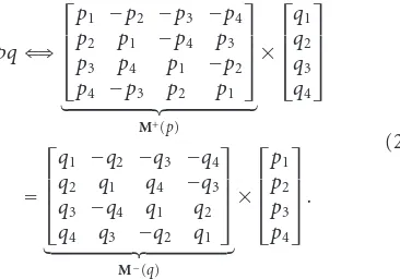
all operations on hypercomplex numbers can be consistently represented in vector-matrix notation. We are particularly interested in multiplication, which can be written in two equivalent forms as
pq⇐⇒
⎡ ⎢ ⎢ ⎢ ⎣
p1 −p2 −p3 −p4 p2 p1 −p4 p3 p3 p4 p1 −p2 p4 −p3 p2 p1
⎤ ⎥ ⎥ ⎥ ⎦
M+(p)
×
⎡ ⎢ ⎢ ⎢ ⎣
q1 q2 q3 q4
⎤ ⎥ ⎥ ⎥ ⎦
=
⎡ ⎢ ⎢ ⎢ ⎣
q1 −q2 −q3 −q4 q2 q1 q4 −q3 q3 −q4 q1 q2 q4 q3 −q2 q1
⎤ ⎥ ⎥ ⎥ ⎦
M−(q)
×
⎡ ⎢ ⎢ ⎢ ⎣
p1 p2 p3 p4
⎤ ⎥ ⎥ ⎥ ⎦.
(27)
Thus two different multiplication matrices exist, the left-M+(·) and right-operandM−(·) one.
In the following discussion, we restrict ourselves to unit quaternion multiplication matrices. To represent quaternion multipliers graphically, we also introduce the symbols shown inFigure 4.
Both matrices are orthogonal as
M±(q)−1=M±(q)T, (28)
and have determinant +1. Hence, they belong to the 4×4 spe-cial orthogonal group commonly referred to as SO(4) [23]. They also form groups with respect to multiplication, which implies the following identities:
M+q
N−1
· · ·M+q 0
=M+q
N−1· · ·q0
, (29a)
M−qN−1
· · ·M−q0
=M−q0· · ·qN−1
. (29b)
Another interesting and useful relation is
M±(q)T=M±(q). (30)
From a PUFB perspective, the connections between quaternion multiplication matrices and arbitrary 4×4 or-thogonal ones are intriguing. To make the paper comprehen-sive, we have decided to repeat the derivations from [24,25]
B q
A
B q
Figure5: Structural transformation corresponding to (31).
in a quite large extent, but the emphasis is placed on slightly different nuances.
3.3. Reduction of a4×4orthogonal matrix
Theorem 1. Every4×4orthogonal matrixAcan be repre-sented as the product
A=M±(a) diag(1,B), (31)
where
a=a11−a21i−a31j−a41k (32)
andBis a3×3orthogonal matrix.
Proof. AsAandM±(a) are both orthogonal,M±(a)TAmust be orthogonal as well. The quaterniona is constructed so as to have the inner product of the first columns ofAand M±(a) equal to unity. This is the value of the (1, 1)st element ofM±(a)TA, so all the remaining elements in the first row and column of this matrix must be zeros. Thus the rest of its elements forms a 3×3 orthogonal matrixB.
The corresponding structural transformation is shown in Figure 5. It should be noted that the reducing ability of unit quaternion multiplication matrices suggests their tight con-nections with Givens rotations, which are commonly used in matrix parameterization via QR decomposition, as it has been mentioned earlier. One quaternion multiplication is re-lated to three degrees of freedom and can be treated as a four-dimensional generalization of a Givens rotation [11].
3.4. Parameterization of a4×4orthogonal matrix
Theorem 2(see [24]). For every orthogonal4×4matrixA, there exists a unique (up to signs) pair of unit quaternions p
andqsuch that
A=M+(p)M−(q)=M−(q)M+(p). (33)
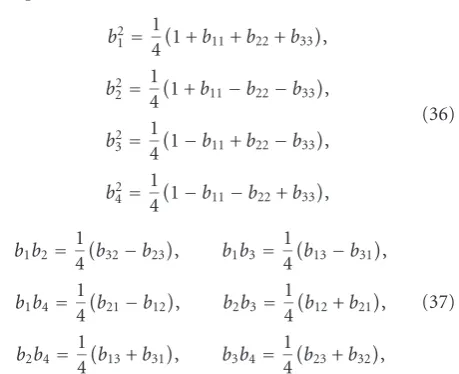
Proof. We begin by decomposing the given matrix A ac-cording to (31) and then deal with diag(1,B). It is known [25] that the latter matrix can be represented using one unit quaternionbas
M+(b)M−(b)=diag(1,B), (34)
where
B=
⎡ ⎢ ⎢ ⎣
b21+b22−b32−b24 2
−b1b4+b2b3
2b1b3+b2b4
2b1b4+b3b2
b2
1−b22+b23−b42 2
−b1b2+b3b4
2−b1b3+b4b2
2b1b2+b4b3
b21−b22−b32+b24
⎤ ⎥ ⎥ ⎦.
The equations
b21=
1 4
1 +b11+b22+b33
,
b22=
1 4
1 +b11−b22−b33
,
b32=
1 4
1−b11+b22−b33
,
b42=
1 4
1−b11−b22+b33
,
(36)
b1b2=1
4
b32−b23
, b1b3= 1
4
b13−b31
,
b1b4=1
4
b21−b12
, b2b3=1
4
b12+b21
,
b2b4=1
4
b13+b31
, b3b4= 1
4
b23+b32
,
(37)
which can be easily derived, allow us to calculatebfromB. This system of equations is overdetermined as the num-ber of equations exceeds the numnum-ber of unknowns. To avoid a contradiction, the equation which gives thebkof a max-imum absolute value should be selected from among (36). Then it must be supplemented by the three equations in (37) which involvebk, to allow us to determine all components of the quaternionb. It should be noted that the squares at the left-hand side of (36) make−ban equivalent solution. Finally, we get the desired factorization
A=M+(a)M+(b)M−(b)=M+(ab)M−(b) (38)
based on the quaternionsp=abandq=b.
It should be emphasized that the matrix product (33) is commutative, though the product of the related quaternions is not. The theorem is also true after the transition to−pand
−q.
3.5. Quaternion multiplier as paraunitary building block
The parameterization (33) has several advantages which make quaternion multipliers interesting paraunitary build-ing blocks.
First of all, a quantized quaternion multiplication matrix, for example,
⎡ ⎢ ⎢ ⎢ ⎣
Qq1
−Qq2
−Qq3
−Qq4
Qq2
Qq1
−Qq4
Qq3
Qq3
Qq4
Qq1
−Qq2
Qq4
−Qq3
Qq2
Qq1
⎤ ⎥ ⎥ ⎥
⎦ (39)
still has the same sets of absolute values in all its rows and columns. So the column norm is constant and is equal to
Q(q1)2+Q(q2)2+Q(q3)2+Q(q4)2, and hence the
prod-uct (33) always represents an orthogonal transformation. Moreover, it is sufficient to hold only 8 real numbers (2 quaternions) in memory, whereas the direct representa-tion of the corresponding matrix would require to store all its 16 entries.
z 1
z 1
z 1 4 4 4 4
p0 q0 z 1 q1 z 1 q2
E0 Λ(z) R1 Λ(z) R2
Figure 6: Quaternionic lattice structure for 4-channel general PUFB (N=3).
The specific structures of quaternion multiplication ma-trices allow us to perform this operation in 8 real multiplica-tions, but the algorithm is quite intricate [26].
The possibility of multiplierless implementations is much more important. They can be realized with distributed arithmetic or using four-dimensional CORDIC algorithm. The feasibility of computation parallelization or pipelining together with the regularity of the layout of a digital circuit make quaternionic multiplier very attractive for FPGA and VLSI technologies [27].
4. QUATERNIONIC LATTICE STRUCTURES
4.1. Four-channel general PUFB
Theorem 3(see [11]). The quaternionic variant of the factor-ization(1)for a4-channel general PUFB results from the fol-lowing substitution:
E0=M+
q0
M−p0
, (40)
Ri=M±qi
, i=1,. . .,N−1, (41)
wherep0and allqiare unit-norm quaternions.
Proof. Both of the theorems from the previous section, which concern 4×4 orthogonal matrices, are exploited. According to (31), the matricesRiin (1) can be represented as
Ri=M±
qi
diag1,Bi
. (42)
Since
diag1,Bi Λ(z)=Λ(z) diag
1,Bi
, (43)
the 3×3 orthogonal matrixBican be moved to the preceding stage and multiplied byRi−1. The same procedure can be
ap-plied to the resulting orthogonal matrix. Starting fromRN−1,
we process the subsequent stages to reach E0 and to apply
(33).
z 1
z 1
z 1 4 4 4 4
J2
q0 p0 1/
2 1/
2 1/
2 1/
2
z 1
z 1
1/2 1/2 1/2 1/2 p1
z 1
z 1
p2 1/2 1/2 1/2 1/2
W Φ0
E0
W Λ(z) W Φ1 G1(z)
W Λ(z) W Φ2 G2(z) Figure7: Quaternionic lattice structure for 4-channel LP PUFB (N=3).
Theorem 4(see [12]). A four-band general PUFB determined by(1)in conjunction with(40)and(41)is one-regular if and only if
p0= ±
1
2o qN−1· · ·q0, (44) under the assumption that the left-operand multiplication ma-trix is used in(41).
Proof. By substitutingE(z) with (1) in (16), and then using (40) and (41), we get
M+q
N−1
· · ·M+q 0
M−p0
o=c0e, (45)
asΛ(1) = I4. A simple analysis of the norms of the factors
in this expression gives the value ofc0. It must be±2 as the
norm ofoequals 2, and those ofeand the rows/columns of the quaternion matrices are unity. Hence, by exploiting (29a) too, we can write
M+qN−1· · ·q0
M−p0
o= ±2e. (46)
This clearly suggests to makep0constrained, so we use (30)
to obtain
M−p0
o= ±2M+qN−1· · ·q0)e. (47)
This matrix-vector expression can be interpreted as the quaternionic equation
op0= ±2qN−1· · ·q0 (48)
in whichp0is unknown. The left multiplication byo/4 leads
to the solution, or (44).
The above result can be easily adapted to the case of the right-operand multiplication matrix in (41). We omit this for brevity reasons.
4.2. Four-channel LP PUFB
Theorem 5(see [28]). The conventional, presented inSection 2.2, factorization for 4-channel LP PUFBs changes into a quaternionic alternative when
Φ
0=M−
p0
M+q
0
, (49)
Φ
i=M−
pi
, i=1,. . .,N−1, (50)
αi
Ui
Vi βi
(a)
Ui=I
Vi βi
(b)
αi
Ui
Vi αi
(c)
Figure8: (a) Conventional, (b) simplified, and (c) quaternionic re-alizations ofΦi.
are used instead of (8). All pi and q0 are unit quaternions
which have the two last imaginary parts (related to jandk) zeroed, so they are constrained to be complex numbers in fact.
Proof. Theorem 2allows us to decompose each matrixΦi de-fined by (8) in the following way:
Φi=M−
pi
M+qi
. (51)
The block-diagonal structure ofΦiis inherited by the quater-nion multiplication matrices and this is the cause of the de-generation of the corresponding hypercomplex numbers to the complex ones. It is easy to check that
M+qi
W=WM+qi
, (52)
M+q
i
Λ(z)=Λ(z)M+q
i
. (53)
ThusM+q
i
can be moved to the preceding stage Gi−1(z),
which leads to (50). As the product Φi−1M+
qi
maintains orthogonality and a block-diagonal structure, the procedure can be repeated on it. The only exception is atΦ0, which
must be represented using both quaternion multiplication matrices.
z 1
z 1
z 1 4 4 4 4
J2
p0 1/
2 1/
2 1/
2 1/
2
z 1
z 1
1/2 1/2 1/2 1/2 p1
z 1
z 1
Γ J2
p2 1/2 1/2 1/2 1/2
W Φ0
E0
W Λ(z) W Φ1 G1(z)
W Λ(z) W Φ2 G2(z) Figure9: Quaternionic lattice structure for 4-channel PMI LP PUFB (N=3).
Theorem 6(see [12]). A 4-band LP PUFB realized using the quaternionic approach is one-regular if and only if
q0= ±
1
√
2p0· · ·pN−1a. (54)
Proof. As in the case of a general PUFB, the first step is to expand (16) in accordance with the considered factorization ofE(z). We get
M−pN−1
· · ·M−p0
M+q
0
√
2a=c0e (55)
asWΛ(1)W=2I4 andWdiag(I2,J2)o=a. The value ofc0
again results from the examination of the norms of the fac-tors and must be±2 as the norm ofaequals√2, while the remaining ones are unity. Applying (29b), we obtain
M−p0· · ·pN−1
M+q
0
a= ±√2e (56)
and see that it is the easiest to make q0 dependent on the
remaining coefficients. The identity (30) allows us to write the matrix equation
M+q 0
a= ±√2M−p0· · ·pN−1
e (57)
and then convert it into the quaternionic equivalent
q0a= ± √
2p0· · ·pN−1. (58)
The right multiplication bya/2 gives the desired regularity constraint (54) onq0.
4.3. Four-channel PMI LP PUFB
Theorem 7(see [28]). The constraints(12)-(13)on the ma-trices used in the factorization fromSection 2.3, for4-channel PMI LP PUFBs, can be satisfied by taking
Φ
i =M−
pi
, i=0,. . .,N−2, (59)
Φ
N−1=M−
pN−1
diagJ2Γ,I2
, (60)
whereΓ=diag(1,−1)and the quaternionic coefficientspiare restricted to be unit complex numbers.
Proof. In the case of 4 channels,ΓViΓ=VTi, and so the first condition (12) necessary to obtain PMI symmetry directly imposes the form ofΦiwhich coincides with a quaternion multiplication matrix, because
Φi=diag
ΓViΓ,Vi
=diagVTi,Vi
M−(pi)
(61)
ifpiis constrained to be a complex number.
The obvious identities JJ = I andJ2ViJ2 = VTi allow
a quaternion multiplication matrix to be extracted also from
ΦN−1determined by the condition (13). Namely,
ΦN−1=diag
J2VN−1Γ,VN−1
=diagVT
N−1,VN−1
M−(pN−1)
diagJ2Γ,I2
. (62)
The corresponding structure is shown inFigure 9. In the case of a PMI LP PUFB, by quaternionic factorization the number of coefficients is decreased with respect to the con-ventional solution and is the same as in its simplification de-rived in [18].
Theorem 8(see [12]). A four-band PMI LP PUFB realized according toTheorem 7is one-regular if and only if
pN−1= ±
1
√
2ap0· · ·pN−2. (63)
Proof. Given the quaternionic factorization, we can expand (16) into
M−pN−1
diagJ2Γ,I2
·M−pN−2
· · ·M−p0
√
2a=c0e.
(64)
The value ofc0results from norm inspection and equals±2.
Noticing that
diagJ2Γ,I2
=1
2M
+(
a)M−(a), (65)
and utilizing (29b) and (30), we can rewrite (64) as
1 2M
+(
a)M−(a)M−p0· · ·pN−2
a= ±√2M−pN−1
e.
Then, the transition to quaternions yields
1
√
22aap0· · ·pN−2a= ±pN−1, (67)
and we obtain (63) by conjugating both sides, asaa=2.
4.4. Robustness to coefficient quantization
All of the developed lattice structures are lossless regard-less of coefficient quantization. This is because the de-rived factorizations contain no components which become nonorthogonal when represented with finite precision. Thus, the frequency responses of such systems are always power-complementary [2]:
M−1
k=0
Hk
ejω2=c2, ∀ω, (68)
thoughccan deviate from 1. If a compensation of this effect is desired,ccan be calculated as
c2=M
−1
k=0
Hk
ejω2
ω=0=
M−1
k=0
L−1
n=0 hk(n)
2
. (69)
and the multiplication by its reciprocal can be easily embed-ded into the computational scheme.
The plot thickens if regularity is considered because the quaternion conditioned by the others under (44), (54), or (63) must be represented accurately. Fortunately, the neces-sary wordlength is finite and strictly determined by those of the remaining coefficients. Moreover, any scaling of the coef-ficient value does not disturb regularity.
To demonstrate that regularity can indeed be easily im-posed on quaternionic lattice structures, even under finite precision, the next section shows three design examples. The obtained filter banks with rational quaternionic coefficients can be implemented using fixed-point arithmetic, possibly in multiplierless manner as in [29].
5. DESIGN EXAMPLES
5.1. Coefficient synthesis methodology
The goal was to obtain frequency-selective filter banks with high coding gains. So, the weighted sum of two criteria was used as an objective function for optimization.
The first criterion is the stopband attenuation measured in terms of energy as
εSBE=
M−1
k=0
ω∈Ωk Hk
ejω2dω, (70)
whereΩkdenotes the stopband of thekth filter and the num-ber of channels,M, equals 4 in our case.
The second performance criterion is a coding gain de-fined as
CG=10 log10(1/M) M−1
k=0 σx2k
M−1
k=0 σx2k
1/M, (71)
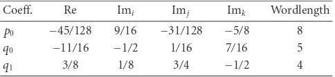
Table1: Rational coefficient values for general PUFB.
Coeff. Re Imi Imj Imk Wordlength
p0 −45/128 9/16 −31/128 −5/8 8
q0 −11/16 −1/2 1/16 7/16 5
q1 3/8 1/8 3/4 −1/2 4
whereσ2
xkare the subband variances. They correspond to the diagonal elements of the autocorrelation matrix of the trans-formed signal,Ry y:
σ2
xk=
Ry y
kk. (72)
It can be determined as the product
Ry y=HRxxHT (73)
of the autocorrelation matrix of the input signal,Rxx, and the transform matrixHformed from the impulse responses of the filter bank as follows:
[H]kn=hk(L−1−n), (74)
wherek=0,. . .,M−1 andn=0,. . .,L−1.
In our experiments, the matrixRxxwas generated for an AR(1) input process with unit variance and the correlation coefficient of 0.95. Such a model is particularly appropriate only for natural images, and therefore other applications will require different approaches.
In the synthesis procedures, the quaternion lattice coef-ficients assumed to be unconstrained in (54) and (63) were represented in the polar form (25). So the standard Matlab routines intended for an unconstrained optimization, that is, fminunc and fminsearch, could be used to search for the angles that minimize the objective function. Given infinite-precision coefficients, we carefully converted them into ra-tionals. This was done intuitively by hand, but the develop-ment of an advanced algorithm, like that proposed in [29], is planned.
5.2. Design example 1: 8-tap general PUFB
A 4-channel 8-tap PUFB was designed using the results from Section 4.1. The synthesized coefficients of quaternionic lat-tice structure are given in Table 1 and the corresponding magnitude responses are shown inFigure 10(a). The filter bank is characterized by a coding gain of 8.1227 dB and a minimum stopband attenuation of 20 dB, so it can com-pete with the similar system demonstrated in [10].
40 30 20 10 0
Hk
(
e
jω)
(dB)
0 0.2 0.4 0.6 0.8 1
ω/π (a)
1 0.5 0 0.5 1
Im
ag
inar
y
par
t
7
2 1 0 1 2
Real part (b)
φ(t) ψ1(t)
ψ2(t) ψ3(t)
(c)
Figure 10: Design example of general PUFB: (a) magnitude re-sponses, (b) zeros of H0(z), and (c) the scaling function and
wavelets.
to the mirror aliasing frequencies.Figure 10(c)demonstrates the wavelet basis related to the system.
5.3. Design example 2: 12-tap LP PUFB
The second design example demonstrates the usefulness of the theory developed inSection 4.2. The hypercomplex coef-ficient values given inTable 2determine the 12-tap LP PUFB which has a coding gain of 8.1845 dB. The plots inFigure 11 allow us to evaluate the magnitude responses of the system and verify its one-regularity. The filters have good frequency selectivity. For the lowpass and highpass ones, the sidelobes are below the−35 dB level, whereas for the bandpass filters, the peak amplitude of the sidelobes is about−20 dB.
Table2: Rational coefficient values for LP PUFB.
Coeff. Re Imi Imj Imk Wordlength
q0 −231/512 459/1024 0 0 11
p0 −7/8 −3/8 0 0 4
p1 −3/16 15/16 0 0 5
p2 −9/16 −13/16 0 0 5
50 40 30 20 10 0
Hk
(
e
jω
)
(dB)
0 0.2 0.4 0.6 0.8 1
ω/π (a)
1 0 1
Im
ag
inar
y
par
t
11
5 4 3 2 1 0 1 2
Real part (b)
φ(t) ψ1(t)
ψ2(t) ψ3(t)
(c)
Figure11: Design example of LP PUFB: (a) magnitude responses, (b) zeros ofH0(z), and (c) the scaling function and wavelets.
5.4. Design example 3: 12-tap PMI LP PUFB
Table3: Rational coefficient values for PMI LP PUFB.
Coeff. Re Imi Imj Imk Wordlength
p0 7/8 3/8 0 0 4
p1 3/16 −1 0 0 5
p2 −17/128 43/64 0 0 8
50 40 30 20 10 0
Hk
(
e
jω
)
(dB)
0 0.2 0.4 0.6 0.8 1
ω/π (a)
1.5 1 0.5 0 0.5 1 1.5
Im
ag
inar
y
par
t
11
4 3 2 1 0 1 2
Real part (b)
φ(t) ψ1(t)
ψ2(t) ψ3(t)
(c)
Figure12: Design example of PMI LP PUFB: (a) magnitude re-sponses, (b) zeros of H0(z), and (c) the scaling function and
wavelets.
−20 dB. The reason for this is the similarity of the zero loca-tions shown inFigure 12(b)to those inFigure 11(b). The dif-ferences between the wavelet bases are almost unnoticeable.
6. CONCLUSION
The developed quaternionic approach to the design and im-plementation of four-band PUFBs seems to be very compet-itive with the conventional techniques. Its unique advantage
is the structural imposition of paraunitary property (lossless-ness) even with finite-precision arithmetic. It also enables the straightforward expression of the one-regularity conditions in terms of the coefficients of the quaternionic lattice struc-ture, which is also advantageous in fixed-point implementa-tions. So the solution is especially interesting from a practical point of view.
ACKNOWLEDGMENTS
This work was supported by the Polish Ministry of Science and Higher Education (MNiSzW) in years 2005-2006 (Grant no. 3 T11F 014 29). It was also partially supported by Bia-lystok Technical University under the Grant W/WI/2/05.
REFERENCES
[1] P. P. Vaidyanathan and Z. Doˇganata, “The Role of lossless systems in modern digital signal processing: a tutorial,”IEEE Transactions on Education, vol. 32, no. 3, pp. 181–197, 1989. [2] P. P. Vaidyanathan, Multirate Systems and Filter Banks,
Prentice-Hall, Englewood Cliffs, NJ, USA, 1993.
[3] P. P. Vaidyanathan, T. Q. Nguyen, Z. Doˇganata, and T. Sara-maki, “Improved technique for design of perfect reconstruc-tion FIR QMF banks with lossless polyphase matrices,”IEEE Transactions on Acoustics, Speech, and Signal Processing, vol. 37, no. 7, pp. 1042–1056, 1989.
[4] A. K. Soman, P. P. Vaidyanathan, and T. Q. Nguyen, “Linear phase paraunitary filter banks: theory, factorizations and de-signs,”IEEE Transactions on Signal Processing, vol. 41, no. 12, pp. 3480–3496, 1993.
[5] A. K. Soman and P. P. Vaidyanathan, “A complete factorization of paraunitary matrices with pairwise mirror-image symmetry in the frequency domain,”IEEE Transactions on Signal Process-ing, vol. 43, no. 4, pp. 1002–1004, 1995.
[6] S. Oraintara, T. D. Tran, P. N. Heller, and T. Q. Nguyen, “Lat-tice structure for regular paraunitary linear-phase filterbanks andM-band orthogonal symmetric wavelets,”IEEE Transac-tions on Signal Processing, vol. 49, no. 11, pp. 2659–2672, 2001. [7] P. P. Vaidyanathan and P.-Q. Hoang, “Lattice structures for op-timal design and robust implementation of two-band perfect reconstruction QMF banks,” IEEE Transactions on Acoustic, Speech, and Signal Processing, vol. 36, no. 1, pp. 81–94, 1988. [8] P. P. Vaidyanathan, “On coefficient-quantization and
com-putational roundoffeffects in lossless multirate filter banks,”
IEEE Transactions on Signal Processing, vol. 39, no. 4, pp. 1006– 1008, 1991.
[9] Y.-J. Chen and K. S. Amaratunga, “M-channel lifting factor-ization of perfect reconstruction filter banks and reversible M-band wavelet transforms,”IEEE Transactions on Circuits and Systems II: Analog and Digital Signal Processing, vol. 50, no. 12, pp. 963–976, 2003.
[10] Y.-J. Chen, S. Oraintara, and K. S. Amaratunga, “Dyadic-based factorizations for regular paraunitary filterbanks and M-band orthogonal wavelets with structural vanishing mo-ments,”IEEE Transactions on Signal Processing, vol. 53, no. 1, pp. 193–207, 2005.
[12] M. Parfieniuk and A. Petrovsky, “Quaternionic formulation of the first regularity for four-band paraunitary filter banks,” in
Proceedings of IEEE International Symposium on Circuits and Systems (ISCAS ’06), pp. 883–886, Kos, Greece, May 2006. [13] Z. Doˇganata, P. P. Vaidyanathan, and T. Q. Nguyen,
“Gen-eral synthesis procedures for FIR lossless transfer matrices, for perfect-reconstruction multirate filter bank applications,”
IEEE Transactions on Acoustics, Speech, and Signal Processing, vol. 36, no. 10, pp. 1561–1574, 1988.
[14] G. Strang and T. Q. Nguyen, Wavelets and Filter Banks, Wellesley-Cambridge Press, Wellesley, Mass, USA, 1996. [15] R. L. de Queiroz, T. Q. Nguyen, and K. R. Rao, “The GenLOT:
generalized linear-phase lapped orthogonal transform,”IEEE Transactions on Signal Processing, vol. 44, no. 3, pp. 497–507, 1996.
[16] L. Gan and K.-K. Ma, “A simplified lattice factorization for linear-phase perfect reconstruction filter bank,”IEEE Signal Processing Letters, vol. 8, no. 7, pp. 207–209, 2001.
[17] T. Q. Nguyen and P. P. Vaidyanathan, “Maximally decimated perfect-reconstruction FIR filter banks with pairwise mirror-image analysis (and synthesis) frequency responses,” IEEE Transactions on Acoustics, Speech, and Signal Processing, vol. 36, no. 5, pp. 693–706, 1988.
[18] L. Gan and K.-K. Ma, “A simplified lattice factorization for linear-phase paraunitary filter banks with pairwise mirror im-age frequency responses,”IEEE Transactions on Circuits and Systems II: Express Briefs, vol. 51, no. 1, pp. 3–7, 2004. [19] O. Rioul, “Regular wavelets: a discrete-time approach,”IEEE
Transactions on Signal Processing, vol. 41, no. 12, pp. 3572– 3579, 1993.
[20] P. Steffen, P. N. Heller, R. A. Gopinath, and C. S. Burrus, “The-ory of regularM-band wavelet bases,”IEEE Transactions on Signal Processing, vol. 41, no. 12, pp. 3497–3511, 1993. [21] W. R. Hamilton, “On quaternions; or on a new system of
imag-inaries in algebra,”The London, Edinburgh and Dublin Philo-sophical Magazine and Journal of Science, vol. 25, pp. 489–495, 1844.
[22] I. L. Kantor and A. S. Solodovnikov,Hypercomplex Numbers: An Elementary Introduction to Algebras, Springer, New York, NY, USA, 1989.
[23] A. Baker,Matrix Groups: An Introduction to Lie Group Theory, Springer, London, UK, 2002.
[24] H. G. Baker, “Quaternions and orthogonal 4x4 real matrices,” Tech. Rep., June 1996, http://www.gamedev.net/reference/ articles/article428.asp.
[25] E. Salamin, “Application of quaternions to computation with rotations,” Tech. Rep., Stanford AI Lab, Stanford, Calif, USA, 1979.
[26] T. D. Howell and J. C. Lafon, “The complexity of the quaternion product,” Tech. Rep. TR 75-245, Cornell Univer-sity, Ithaca, NY, USA, June 1975,http://citeseer.ist.psu.edu/ howell75complexity.html.
[27] M. Parfieniuk and A. Petrovsky, “Implementation perspectives of quaternionic component for paraunitary filter banks,” in
Proceedings of the International Workshop on Spectral Methods and Multirate Signal Processing (SMMSP ’04), pp. 151–158, Vi-enna, Austria, September 2004.
[28] M. Parfieniuk and A. Petrovsky, “Linear phase paraunitary fil-ter banks based on quafil-ternionic component,” inProceedings of International Conference on Signals and Electronic Systems (IC-SES ’04), pp. 203–206, Pozna ´n, Poland, September 2004.
[29] Y.-J. Chen, S. Oraintara, T. D. Tran, K. Amaratunga, and T. Q. Nguyen, “Multiplierless approximation of transforms with adder constraint,”IEEE Signal Processing Letters, vol. 9, no. 11, pp. 344–347, 2002.
Marek Parfieniuk was born in Bialystok, Poland, in 1975. He received his M.S. degree in computer science, with honors, from Bi-alystok Technical University, in 2000. Cur-rently, he is completing the procedures for the Ph.D. degree. Since 2000, he has been an Assistant Lecturer at Faculty of Com-puter Science, Bialystok Technical Univer-sity. From 2000 to 2003, he also worked for ComputerLand S.A. as an Enterprise Soft-ware Developer.
Alexander Petrovsky received the Dipl.-Ing. degree in computer engineering, in 1975, and the Ph.D. degree, in 1980, both from the Minsk Radio-Engineering Insti-tute, Minsk, Belarus. In 1989, he received the Doctor of Science degree from The In-stitute of Simulation Problems in Power Engineering, Academy of Science, Kiev, Ukraine. In 1975, he joined Minsk Radio-Engineering Institute. He became a