A shrinkage probability hypothesis density filter for multitarget tracking

R E S E A R C H

Open Access

A shrinkage probability hypothesis density filter

for multitarget tracking

Huisi Tong

, Hao Zhang, Huadong Meng and Xiqin Wang

Abstract

In radar systems, tracking targets in low signal-to-noise ratio (SNR) environments is a very important task. There are some algorithms designed for multitarget tracking. Their performances, however, are not satisfactory in low SNR environments. Track-before-detect (TBD) algorithms have been developed as a class of improved methods for tracking in low SNR environments. However, multitarget TBD is still an open issue. In this article, multitarget TBD measurements are modeled, and a highly efficient filter in the framework of finite set statistics (FISST) is designed. Then, the probability hypothesis density (PHD) filter is applied to multitarget TBD. Indeed, to solve the problem of the target and noise not being separated correctly when the SNR is low, a shrinkage-PHD filter is derived, and the optimal parameter for shrinkage operation is obtained by certain optimization procedures. Through simulation results, it is shown that our method can track targets with high accuracy by taking advantage of shrinkage operations.

Keywords:multi-target tracking, track-before-detect, PHD filter

1 Introduction

In order to extract target measurements, traditional tracking methods apply a detection threshold at every scan. The undesirable effect of detecting is that useful information is thrown away potentially in restricting the data flow. For high signal-to-noise ratio (SNR) targets, this loss of information is of little concern [1]. For low SNR targets, this loss of information could be critical for a radar tracking system. Therefore, some new algorithms using unthresholded data are more advantageous than the traditional methods in tracking low SNR targets.

The concept of simultaneous detection and tracking using unthresholded data is known in the literature as track-before-detect (TBD) approach [1]. TBD algorithms could improve the performance of a tracking system, which has been investigated for surveillance radar [2]. In [3,4], the advantage of TBD methods is discussed and many TBD methods are reviewed and compared. As a batch algorithm using the Hough transform [5], dynamic programming [6] or maximum likelihood estimation [7], TBD could be implemented. These techniques operate

on several data scans and, in general, require large com-putational resources [1].

As an alternative, recursive TBD method is based on a recursive single-target Bayes filter [1]. An extension of the particle filter to multitarget TBD is given in [8], and an improved approach is given in [9]. In this algorithm, a modeling setup is applied to accommodate the varying number of targets. Then, a multiple model Sequential Monte Carlo-based TBD approach is used to solve the problem conditioned on the model, i.e., the number of targets [10]. This approach has proven to be very efficient in both single and multitarget cases [3], though it restricts itself to the case in which the maximum possible number of targets is limited and known.

Another extension of the single-target Bayes filter to multitarget TBD is based on a multitarget Bayes filter. Because a single-target Bayes filter is optimal for a single target, to solve the problems introduced by multiple tar-gets, the multitarget Bayes filter is proposed in [11]. In a multitarget Bayes filter, multitarget states and observa-tions are modeled as random finite sets (RFS). This approach is a theoretically optimal approach to multitar-get tracking in the framework of finite set statistics (FISST) [12]. However, the multitarget Bayes filter has no practical utility without an approximation strategy. To * Correspondence: [email protected]

Department of Electronic Engineering, Tsinghua University Beijing, People’s Republic of China

solve this problem, the probability hypothesis density (PHD) filter [13] is proposed as a tractable and calcula-tion-simple alternative to the multitarget Bayes filter [14]. The PHD is the first moment of the multitarget poster-ior probability. Under some assumptions (e.g., Poisson Assumption), the PHD is an approximation of the multi-target posterior probability. Therefore, the PHD filter can be an approximation of the multitarget Bayes filter. Although a PHD algorithm for TBD is proposed in [10], this approach ignores TBD measurements should be modeled by RFSs. In [15], multitarget TBD from image observations is formulated in a Bayesian framework by modeling the collection of states as a multi-Bernoulli RFS. This work use the multi-Bernoulli update to develop a high precision multi-object filtering algorithm for image observations, although its adaptability of low SNR environment is needed to discussed in more detail.

In our previous work [16], we use the RFSs to model multitarget TBD measurements and the collection of states. In this way, a traditional PHD filter [12,13] could be applied to multitarget TBD. Even though PHD could be an approximation of the multitarget posterior probability, the accuracy of the algorithm is limited by some reasons, which are indicated in this article. First, when the SNR is too low, the PHD cannot be a sufficient approximation of the multitarget posterior probability because the funda-mental assumptions are challenged. Furthermore, for mul-titarget TBD, the measurements of target and noise can hardly be separated, while the PHD filter is heavily depen-dent on the measurements of targets [17]. In traditional tracking systems, to solve these problems, cardinalized PHD filter (CPHDF) is proposed in [18]. However, CPHDF is inefficient in multitarget TBD, because the computational complexity of CPHDF isO(m3

), where m is the number of elements of the measurement set and is quite large for the TBD problem.

In this article, for extending a traditional PHD filter to be suitable for multitarget TBD, viewed from a different perspective, TBD can be regarded as a kind of classifica-tion problem of target and noise measurements. To enhance the difference between the target and noise mea-surements and to pursue better classification perfor-mance, the measurements need to be denoised. The threshold shrinkage algorithm [19] is an important method for image denois-ing. In general, the key points of threshold shrinkage are the following: the method of shrinkage (e.g., soft-threshold method) and the selection criterion of the threshold. In this article, a shrinkage operation is adopted that is similar to the threshold shrinkage algorithm. The optimal parameter for the shrinkage operation can be obtained via certain optimiza-tion procedures.

Furthermore, in this article, some problems of multitar-get TBD in particle use are also discussed. The assumption

of known SNRs is used frequently in traditional TBD algo-rithms [6,8,9]. Multiple targets with similar SNRs are com-mon assumption in the simulations of PHD algorithms using the amplitude feature, as in [15,20]. However, in practical use, multiple targets with different or unknown SNRs are common. In this article, for the sequential Monte Carlo (SMC) implement of the PHD filter adopted, this problem could be solved by augmenting the SNR into target state, varying the method of generating predicted particles and adjusting the update operator.

In this article, the measurement of targets is modeled by a‘nail-like’model on range-Doppler maps because of the assumptions of the classical PHD filter in the frame-work of FISST. Recently, a classical PHD filter has been modified to solve the problems of extended and group targets in [21,22], respectively. Therefore, the TBD mea-surement model of extended targets in the framework of FISST will be discussed in future work.

The rest of this article is organized as follows: in Section 2, the multitarget TBD problem is modeled by RFSs. In Section3, the limitation of traditional PHD filter extension to TBD is investigated. In Section 4, a shrinkage option for the PHD filter is proposed with an optimal parameter. Tracking multiple targets with different or unknown SNRs is discussed in Section 5. Simulation results for the track-ing systems are presented in Section 6, and finally, we con-clude the article in Section 7.

2 Multitarget TBD RFS model

2.1 State of the RFS model

The target state is xk=

xk,x˙k,yk,y˙k

T

, where (xk,yk) and

˙ xk,y˙k

are the position and velocity. Since there is no ordering on the respective collections of all target states, they can be naturally represented as a finite set.Xkis the multitarget state-set at time step k, i.e., the set of unknown target states (which are also of unknown number).

In a single-target scenario, the state xkis modeled as random vectors. Then, the multitarget state, including target motion, birth, spawning, can be described by RFS. For target motion, given multitarget state setXk-1, each xk-1 Î Xk-1 either survives at time step k with probabilityek|k-1(xk-1), and its transition probability den-sity fromxk-1 toxkis fk|k-1(xk|xk-1). Therefore, the target motion is modeled as the RFSSk|k-1(xk-1). In the same way, when the RFS of target birth at timek is modeled by Γk, and the RFS of targets spawning from a target with xk-1is modeled by Bk|k-1(xk-1), the multitarget stat Xkis given by

Xk=

∪

xk−1∈Xk−1

Sk|k−1(xk−1)

∪

∪

xk−1∈Xk−1

Bk|k−1(xk−1)

2.2 Measurement of the RFS model

The measurements are measurements of reflected power as in [8].nkis white complex Gaussian noise with var-iance σ02. In this section, assume that the intensity of all

targets isIk, the SNR for the targets is defined by

SNR = 10 log

I_k2

2σ₀2 dB. (2)

The method to deal with multiple targets with differ-ent or unknown SNRs is discussed in Section 5.

Because of the assumptions made in the modeling process and the essential difference between an RFS and a random vector, the two conditions that should be satisfied to model TBD measurements by a RFS are the following: there is no target that generates more than one measurement vector, and no measurement vector is generated by more than one target [21]. In summary, the measurement of targets should be modeled by a ‘nail-like’ model on the range-Doppler-Bearing maps [theijkcell is defined by coordinate (ri,dj,bl)] as follow:

R, Dand B are the size of a range, the Doppler and

the bearing cell. rk=

(xk)2+ (yk)2,dk=

xkx˙k+yk˙yk

(xk)2+ (yk)2

and bk= arctan

yk

xk

·Rik=

ri−R₂,ri+R₂

,Djk=

dj−D₂,dj+D₂

and Bl_k=bl−B₂,bl+B₂

.

Then, the measurement model is

zijl_k =hijl(xk) +nk

2

(3)

hijl=

Ikifrk∈Ri_k, dk∈Dj_kandbk∈Bl_k

0 else (4)

This means the measurement of a target is like a nail on the range-Doppler-bearing maps. This ‘nail-like’ model is similar to the point target model in [5,6]. At stepk, the measurement provided by the sensor consists of N=Nr ×Nd×Nbmeasurements zijl_k , whereNr, Nd andNbare the number of range, Doppler and bearing cells.

The number of zijl_k is a constant N. However, the number of element of an RFS should be random and Poisson distributed for a PHD filter. Because weak signal information should be preserved by TBD algorithms, we should make sure all measurements produced by targets are included in the RFS.

Therefore, a threshold could be chosen as follows:

θk= arg min

θk

+∞

θk

g0(zijl_k)dzijl_k

s.t. pD(xk) =P(zijl_k ≥θk) =

+∞

θk

gk(zijl_k|xk)dzijl_k ≥0.99

(5)

where the likelihood function for the target is

gk(z ijl k|xk) =

1 2σ2

0

exp

−z

ijl k +I2k

2σ2 0

I0 ⎛ ⎜ ⎝Ik

zijl_k

σ2 0

⎞ ⎟

⎠ (6)

and that for noise is

p0(zijl_k) =

1 2σ2

0

exp

− 1

2σ2 0

zijl_k

. (7)

where Io() is the zero order Bessel function and zijl_k is assumed positive. The pD(xk) is the probability detec-tion. Because this algorithm is for TBD, it should be ensured thatpD(xk)≈1.

Zkis the observation-set consisting of all measurements collected by all sensors at time-stepk, no matter the mea-surement from the targets or from the noise. If zijl_k ≥θk,

letzk=zijl_k . Then, the measurement RFSZkis constructed by a subset of the zijl_k using a thresholding mechanism. The threshold can insure that pD(xk) ≈ 1 by (5). The threshold is a function of the SNR of the targets. The ele-ment in the RFSZkis as follows:

z∗_k= [ri,dj,bl,zk]T (8)

and the likelihood function according

g∗_k(z∗_k|xk)≈gk(zk|xk) (9)

p∗₀(z∗_k) = 1 2σ₀2exp

−zk−θk

2σ₀2

(10)

At the same time, the sensor could be modeled by

Zk=Kk∪

∪

xk∈Xk k(xk)

, z∗_k∈Zk (11)

is shown that when the measurements of TBD are mod-eled by RFSs, multitarget TBD can be regarded as a kind of classification problem of target and noise mea-surements for one scan. This classification problem will be further analyzed in Section 4.

3 The traditional PHD filter extension to TBD After multitarget TBD measurements and the collection of states are modeled by RFS, a traditional PHD filter is applied to multitarget TBD. This algorithm is reviewed in Section 3.1. However, the accuracy of the algorithm is lim-ited by some reasons when the SNR is low, which is dis-cussed in Section 3.2.

3.1 The algorithm

As proposed in [13], the PHD prediction and update equations are presented as follows:

Dk|k−1(x|Z1:k−1) =

ek|k−1(ζ)fk(x|ζ)Dk−1|k−1(ζ|Z1:k−1)dζ +

bk|k−1(x|ζ)Dk−1|k−1(ζ|Z1:k−1)dζ+γk(x)

(12)

Dk|k(x|Z1:k) = [1−pD(x)]Dk|k−1(x) +

zk∈Zk

pD(x)gk(zk|x)Dk|k−1(x)

kk(zk) +

pD(ζ)gk(zk|ζ)Dk|k−1(ζ)dζ (13)

whereDk|k(x|Z1:k) the PHD is the density whose inte-gral ∫S Dk|k(x|Z1:k)dx on any region S of state space is

ˆ

nk(S) =∫ |X∩S|pk(Xk|Z1:k)δX.bk|k−1(xk|xk−1) and gk(xk) denote the intensity ofBk|k-1(xk-1) and Γk at timek, and k(zk) is the intensity ofKk. Z1:kis the time-sequence of observation-sets.

Because the PHD propagation equations involve mul-tiple integrals that have no computationally tractable closed-form expression, sequential Monte Carlo (SMC) methods are used to approximate the PHD in [12]. Let the update PHD atk- 1 stepDk-1|k-1(x|Z1:k-1) be repre-sented by a set of particles {w(_kp₋)₁,x_k(p₋)₁}Lk−1

p=1, as Dk−1|k−1(x|Z1:k) =

Lk−1

p=1

w∗_k(₋p₁)δ(x−x(_kp₋)₁) (14) The predicted particles are generated by

x(_kp_|)_k−1∼

qk

•x(_kp₋)₁ p= 1,. . .,Lk−1 vk(•) p=Lk−1+ 1,. . .,Lk−1+Jk

(15)

where qk(•|x_k(p₋)₁) and vk(•) are proposal density. The predicted density is

Dk|k−1(x|Z1:k−1) =

Lk−1+Jk

p=1

w(_kp_|k)₋₁δ(x−x(_kp_|k)₋₁) (16)

where

w(_kp_|k)₋₁=

⎧ ⎪ ⎪ ⎪ ⎪ ⎪ ⎪ ⎪ ⎪ ⎪ ⎨ ⎪ ⎪ ⎪ ⎪ ⎪ ⎪ ⎪ ⎪ ⎪ ⎩

ek|k−1(x(kp−)1)fk(x(kp|k)−1x (p)

k−1) +bk|k−1(x(kp|k)−1x (p) k−1)

qk(x(kp|k)−1x (p) k−1)

p= 1,. . .,Lk−1

γk(x(kp|k)−1)

vk(x(kp|k)−1)

p=Lk−1+ 1,. . .,Lk−1+Jk

(17)

SetpD(x)≡1, the update density will be

Dk|k(x|Z1:k) = Lk−1+Jk

p=1

ω∗(p)

k δ(x−x

(p)

k|k−1) (18)

where

ω∗(p)

k =

zk∈Zk

g_k∗(z∗_kx_k(_|p_k)₋₁)ω(_kp_|k)₋₁

kk(zk) + Lk−1+Jk

p=1

g_k∗(z∗_kx_k(_|p_k)₋₁)ω_k(p_|k)₋₁ (19)

According to the standard treatment of particle filter, resample _{ω∗_k(p)/nˆk,x(kp|k)−1}

Lk−1+Jk

p=1 to get {ω (p)

k /nˆk,x(kp)} Lk

p=1.

3.2 The limitation

Becausekk(zk) can be presented by the number of noise samples lk multiplying the clutter probability density, the update operator (19) turns into

ω∗(p) k =

z∗k∈Zk

g∗_kz∗_kx(_kp_|k)₋₁

λkp∗0(zk:σ0) + Lk−1+Jk

p=1

gk∗

z∗_kx_k(p_|k)₋₁ω(p) k|k−1

ω(p)

k|k−1 (20)

p∗₀(zk:σ) =

1 2σ2exp

−zk−θk

2σ2

(21)

λk=Nexp

− θk

2σ2 0

. (22)

WhenNis large and lkis relatively small, the Poisson distribution could be approximated by the distribution of a number of noise samples. However, this approxima-tion will be destroyed whenlkbecome sufficiently large, which is the case in low SNR scenarios, as in Table 1.

When s0 in (20) cannot make PHD a sufficient approximation of the multi-target posterior probability, choosing the“optimal” sbecomes the key problem for extending the PHD filter to be applied in TBD. As dis-cussed in the following section, this selection can be considered as a shrinkage operation, and the optimal parameter for the shrinkage operation can be obtained via certain optimization procedures.

4 Shrinkage operation for TBD

To determine the“optimal”sand make the noise and targets distinguishable, a different perspective should be taken. As referred to in Section 2.2, TBD can be regarded as a kind of classification problem for target and noise measurements. In other words, when a measurement is obtained, should it be classified into a target class or a noise class? To solve this problem, the Fisher class separ-ability criterion, as a supplement of to the traditional Bayesian framework, was adopted in our design for the extension of the PHD filter. Furthermore, to enhance the difference between the target and noise measurements and pursue the better performance of classification, some attempts to reduce the noise are needed. The threshold shrinkage algorithm [19] is an important method for the image denoising. In general, the cores of threshold shrinkage are as follows: the method of shrinkage and the selection criterion of the threshold. A shrinkage opera-tion is adopted in this secopera-tion that is similar to the threshold shrinkage algorithm to some extent. The opti-mal parameter for the shrinkage operation, which acts as the threshold, can be obtained via certain optimization procedures. The PHD filter with the shrinkage operation is called the Shrinkage-PHD filter.

4.1 Fisher class separability criterion

It is known that the Bayesian classifier is the optimal classifier when the posterior probability can be calcu-lated. However, as indicated in Section 3.2, the PHD cannot be a sufficient approximation of multitarget pos-terior probability when the SNR of the targets is low. Therefore, another classification criterion, the Fisher

class separability criterion, is introduced into our methods.

The separation between the two classes of objects defined by Fisher is the ratio of the distance between the centers of classes to the scattering of the classes [23]:

S= d

2 between d2

within

= (μ1−μ

∗

0)2 d2

1+d∗ 2 0

(23)

where μi represents the centers of classes and d2i

denotes the scattering of the classes. In our analysis, they are set to the mean and variance of the likelihood functions of the target and the noise, respectively.

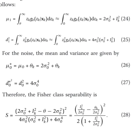
For targets, the mean and variance are defined as follows:

μ1=

∞

θ zkgk(zk|xk)dzk≈

∞

0

zkgk(zk|xk)dzk= 2σ02+I2k(24)

d21= _∞

θ z 2

kgk(zk|xk)dzk≈

_∞

0

z2kgk(zk|xk)dzk= 4σ02(σ02+I2k) (25) For the noise, the mean and variance are given by

μ∗

0=μ0+θk= 2σ02+θk (26)

d∗₀2=d2₀= 4σ₀4 (27)

Therefore, the Fisher class separability is

S= (2σ

2

0 +Ik2−θ−2σ02) 2

4σ2

0(σ02+I2k) + 4σ04

=

I2 k

2σ2 0 −

θk

2σ2 0

2

21 + Ik2

2σ2 0

. (28)

Simulations indicated that the correlation between S

and the SNR of the targets is a positive, approximately linear relationship (as shown in Figure 1). Therefore, when the SNR is low, the Fisher class separability is so small that the targets and false alarms could not be dis-tinguished. In other words, we should enlarge the Fisher class separability of the target class and the noise class when the SNR of the targets is low.

4.2 Shrinkage operation

To enlarge the Fisher class separability between targets and noise, some kind of“shrinkage”operation is applied to the likelihood function of the noise. That is, the para-meter σ₀2in (26) and (27) is adjusted. Ifss≤s0is chosen instead ofσ02itself, then Fisher class separability becomes

Ss=

(2σ2

0 +I2k−θ−2σs2)

2

4σ2

0(σ02+Ik2) + 4σs4

(29) Table 1lversus SNR (N= 2000)

SNR (dB) 6 7 8 9 10

Obviously,Ssis larger than S whenever ss ≤ s0. The following question naturally arises: how does one choose the “optimal” ss, which is the key parameter for the shrinkage process?

4.3 The optimal parameter for the shrinkage operation To demonstrate how influences the classification pro-blem of target and noise measurements, we can define the Mahalanobis distance [23] of measurementzk using the center of the noise class and the target class, respec-tively:

Ss0(zk,σs) =

(zk−θk−2σs2)

2

4σ4

s

(30)

and

Ss1(zk) =

(zk−2σ02−Ik2)

2

4σ2

0(σ02+I2k)

(31)

Because the selection of the threshold is a difficult task for the threshold shrinkage algorithm [19] in the field of image denoising, the selection of the optimal parameter for the shrinkage-PHD filter involves similar problems. For the threshold shrinkage algorithm, an oversized threshold may result in the loss of signal. In contrast, too much noise may remain if an undersized threshold is used. In the same way, for the shrinkage-PHD filter, preserving the weak target information and reducing the noise by tracking are the major challenges to be addressed for TBD problems. Therefore, when considering the two sides, the selection criterion should be designed as follows:

σM

s = max σs

s.t.

⎧ ⎨ ⎩

σs≤σ0 zs

0 gk(zk|xk)dzk=β Ss0(zs,σs)>Ss1(zs)

(32)

The first constraint represents the “shrinkage”. To preserve the weak target information and classify as many low SNR targets to the target class as possible, the Mahalanobis distance of measurement with the center of noise class should be enhanced; hence, the variance of the noise class should be reduced.

The second constraint refers to the fixed probability of target loss. The reason for this term is that for TBD problems, false alarms can be reduced by integration over time. Meanwhile, if target loss occurred, the inte-gration of the information of targets is broken off. Hence, the cost of target loss is much larger than the cost of false alarms, which is the main difference between TBD and common radar detection. Moreover, for the PHD filter, a missed detection can result in loss of the track [17]. Therefore, target loss should be fixed asb. When thebis set, a critical valuezsis determined.

The third constraint means that the measurements zk determined by the second constraint should be classified as targets. When the SNR is low,Ss0(zs,ss) always inter-sects Ss1(zs), so the optimal solution σsM to (32) is

deduced, as indicated in Figure 2a. With the increasing SNR, Ss0(zs,ss) becomes much larger than Ss1(zs) and thus we choose σsM=σ0, as shown in Figure 2b.

Note that although the shrinkage operation could highlight the target measurement and reduce the possi-bility of losing the target during tracking, the noise might be incorrectly increased unavoidably. To mini-mize the influence of shrinkage on the classification of the noise measurement, the maximumss, which is con-sistent with the above constraints, is obtained. The opti-mal solutions to (32) under different SNRs are listed in Table 2.

The update operator of the shrinkage-PHD filter can be summarized as follows:

w∗_k(_,sp)= z∗_k∈Zk

g_k∗(z∗_kx_k(_|p_k)₋₁)ω(_kp_|k)₋₁

λp∗₀(zk:σsM) + Lk−1+Jk

p=1

g_k∗(z∗_kx_k|k−(p) ₁)ω(_k|k−p) ₁ (33)

where σM

s should be set according to Table 2.

5 Multitarget TBD in practical use

This section is to solve of the problem of tracking mul-tiple targets with different or unknown SNRs.

As proposed in Section 4, the optimal parameter for the shrinkage operation is closely related to the SNRs of the target, and the SNRs of the target are assumed to be known and similar. However, in practical use, multiple targets with different or unknown SNRs are common. The PHD is the first moment of the multitarget poster-ior probability, but not the posterposter-ior probability of a

6 7 8 9 10 11 12 13

1 1.5 2 2.5 3 3.5

SNR(dB)

S

certain target. Therefore, the Ik in (6) and the σsM in

Table 2 are difficult to determine. Because the SMC implement of the PHD filter is adopted, this problem could be solved by adjusting the method of generating predicted particles and the update operator.

To describe how to deal with the different SNRs of multiple targets, we augmentIkintoxk:

xk= [x˜k,Ik]T (34)

where x˜k= [xk,x˙k,yk,˙yk]. The particle of the target

state is x(_kp)= [x˜(_kp),I_k(p)]T. The x˜(_kp_|k)₋₁ is generated as 15

˜ x(_kp_|k)₋₁∼

qk(•x˜_k(p₋)₁) p= 1,. . .,Lk−1 vk(•) p=Lk−1+ 1,. . .,Lk−1+Jk

(35)

The I(_kp) is generated by the assumption of a uniform distribution in the range of I˜k, where the SNRs of all of

the targets are [SNR1,SNR2, ...,SNRm], and

Figure 2The Mahalanobis distance versusss: (a) SNR = 8dB; (b) SNR = 13dB.

Table 2 σ_sM (b≤0.05,s0= 0.25)

SNR (dB) 6 7 8 9 10 11 12 13 σM

corresponding to ˜Ik= [I(k,1),I(k,2),. . .,I(k,m)] by

SNRm= 10 log

I2

(k,m)

2σ₀2 dB (36)

In the update operator, because σM

s is a function of

the SNR, it becomes _σM s (I

(p)

k ) in (33).

Note that the θk in (5) should also be adjusted. Because weak signal information should be preserved by TBD algorithms, theIkin (6) is the minimum of ˜Ik.

For the targets with unknown SNRs, it is assumed that the range of the SNRs of the targets is [SNRl, SNRh], corresponding to [I(k,l),I(k,h)]. The I(_kp) could be normal-ized for the region [I(k,l),I(k,h)]. The update operator and threshold are similar to those of multiple targets with different SNRs.

6 Simulation

6.1 Multiple targets miss distance

The optimal sub-pattern assignment (OSPA) distance [15] between the estimated and true multitarget state is adopted here to estimate error.

The OSPA distance is defined as follows [15]. Letd(c)

(q,y): = min(c, ||q- y||) for q, y∈ d, andΠpdenote the set of permutations on {1, 2,..., p} for any positive integerp.cis the cut-off value. Then, forQ= {q1,...,qm} andY= {y1,...,yn},

¯

d(c)(Q,Y) :=1 n

min

π∈n

m

i=1

d(c)(qi,yπ(i)) +c∗(n−m) (37)

if m ≤ n; and d¯(c)_{(Q,Y) :=d}¯(c)_{(Y,Q) if m >n; and}

¯

d(c)_{(Q,Y) =d}¯(c)_{(Y,Q) = 0 ifm=n= 0.}

For example, whenm= 1 andn= 2,Q1= {q1} and Y1 = {y1,y2}, the d¯(c)(Q1,Y1) = 0.5∗(min(min(|q1−y1|,c), min(|q1−y2|,c)) +c).

6.2 Multiple targets with the same SNR

Consider range cells in the interval [80000, 90000] with meters as the unit and Doppler cells in the interval [-400, -150] with meters/second as the unit. Nr = 200,

Nd = 10 andNb = 1. The size of a range and Doppler cell is as follows: R= 50 m andD= 25 m/s. Lk= 2000 andJk= 800. The time intervalTis equal to 1 s.

At time step 1, the first target appears with the initial target state

89000−200 0 0T.

At step 10, a secondary target spawns from the first target, moving at -300 m/s in thex-direction. The stan-dard deviation of the noise is 0.25. In the first example, the SNRs of both targets are 9 dB. The measurements are shown in Figure 3. Tracking with the shrinkage-PHD filter, we plot the shrinkage-PHD of the position and velocity versus time in Figures 4 and 5. It is shown that the PHD of targets can be integrated over time by simulta-neous detection and tracking. Observe that both trajec-tories are automatically initiated and tracked. In step 3, the first target can be tracked stably. At step 11, just 1s after target spawning, the second target is already initiated and tracked.

For the second example, we conducted simulations to compare the performance of the shrinkage-PHD

0

2

4

6

8

10

0

50

100

150

200

0

0.5

1

Doppler cell

Range cell

Poweer

The second target

The first target

filter (shrinkage-PHDF), the PHD filter (PHDF) [16], and the classical multitarget particle filtering method (MPF) [8] in tracking accurately and consistently, and 50 Monte Carlo runs for the same scenario as used in

the first example were performed. The states of targets are estimated by expectation-maximization (EM) algo-rithm. In addition, the maximum possible number of targets is limited and known for MPF, but unlimited

5

10

15

20

8.2

8.3

8.4

8.5

8.6

8.7

8.8

8.9

x 10

0

1

2

x 10

time(s)

position(m)

PHD

Figure 4PHD as a function of position and time step, using the shrink-PHD filter.

5

10

15

20

−400

−350

−300

−250

−200

−150

0

1

2

x 10

time(s)

velocity(m/s)

PHD

and unknown for the PHD filter and the shrinkage-PHDF.

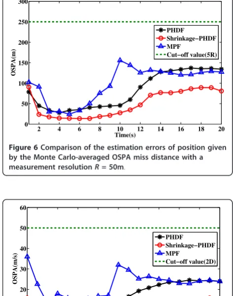
To measure the estimation quantitatively, the estima-tion errors in terms of Monte Carlo averaged OSPA dis-tance are shown in Figures 6 and 7. For position estimation, the cut-off value cis five times the size of the range cell. For velocity estimation, the cut-off value

c is two times the size of the velocity cell. It is shown that the shrinkage-PHDF estimates target position and velocity on all tracks with higher estimated precision than the MPF, because MPF requires a modeling setup to accommodate varying numbers of targets, which is very difficult to accomplish in reality. It also shows that the performance of shrinkage-PHDF is better than PHDF, which is discussed further below.

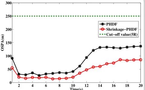
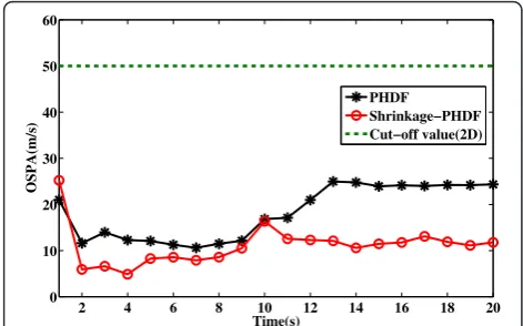
To compare the shrinkage-PHDF and the PHDF clearly, Figures 8 and 9 show the comparison of the mean OSPA for varying SNRs. The SNR of the targets is set to known values between 6 and 13dB. When the value is between 6

2 4 6 8 10 12 14 16 18 20

0 50 100 150 200 250 300

Time(s)

OSPA(m)

PHDF Shrinkage−PHDF MPF

Cut−off value(5R)

Figure 6Comparison of the estimation errors of position given by the Monte Carlo-averaged OSPA miss distance with a measurement resolutionR= 50m.

2 4 6 8 10 12 14 16 18 20

0 10 20 30 40 50 60

Time(s)

OSPA(m/s)

PHDF Shrinkage−PHDF MPF

Cut−off value(2D)

Figure 7Comparison of the estimation errors of the velocity given by the Monte Carlo-averaged OSPA miss distance with a measurement resolution_D= 25m/s.

6 7 8 9 10 11 12 13 0

50 100 150 200 250 300

SNR(dB)

Mean OSPA(m)

PHDF

Shrinkage−PHDF MPF

Cut−off value(5R)

Figure 8Comparison of the estimation errors of position given by the time-averaged OSPA miss distance with a measurement resolutionR= 50m for varying SNRs.

6 7 8 9 10 11 12 13 0

10 20 30 40 50 60

SNR(dB)

Mean OSPA(m/s)

PHDF

Shrinkage−PHDF MPF

Cut−off value(2D)

Figure 9Comparison of the estimation errors of the velocity given by the time-averaged OSPA miss distance with a measurement resolutionD= 25m/s for varying SNRs.

2 4 6 8 10 12 14 16 18 20

0 50 100 150 200 250 300

Time(s)

OSPA(m)

PHDF Shrinkage−PHDF MPF

Cut−off value(5R)

and 11dB, the shrinkage-PHDF performs significantly bet-ter than the PHDF. When the value is large than 11 dB, they perform similarly. This finding illustrates the limita-tion of ordinary the PHDF for TBD: the PHD cannot suffi-ciently approximate the multitarget posterior probability when the SNR is low. The superiority of the shrinkage-PHDF takes advantage of the shrinkage operation is

indicated, especially for low SNR scenarios. It is clear that for multitarget TBD, the shrinkage-PHDF performs better than the PHDF and MPF, especially when the SNR is low.

6.3 Multiple targets with different SNRs

In this example, the targets with different SNRs (the first target is 8 dB, the second target is 9 dB and the last one is 10 dB). At time step 1, the first target appears as in the first example. At step 7, the second target spawns form the first one, and the velocity in the x -direction is -300 m/s. The third target new-birth far from the previous two targets at the time step 13 with the initial target state [89000 -250 0 0]T. A comparison of the estimation errors of the position and the velocity of the three algorithms is shown in Figures 10 and 11. In this scene, the targets vary not only the value of SNRs but also the average number of targets. Because the SNR of the first target is lower than which in Sec-tion 6.2, the convergence velocity of the estimaSec-tion first target is slower. After time step 7, comparing Figures 6 and 10, Figures 7 and 11, the varying SNRs and the number of the targets did not significantly influence the performance of the PHDF and shrinkage-PHDF. In this example, the performance of MPF is better than that in 2 4 6 8 10 12 14 16 18 20

0 10 20 30 40 50 60

Time(s)

OSPA(m/s)

PHDF

Shrinkage−PHDF MPF

Cut−off value(2D)

Figure 11Comparison of the estimation errors of the velocity given by the Monte Carlo-averaged OSPA miss distance for multiple targets with different SNRs (8, 9 and 10dB).

2

4

6

8

10

12

14

16

18

20

0

50

100

150

200

250

300

Time(s)

OSPA

(m

)

PHDF

Shrinkage−PHDF

Cut−off value(5R)

the first example. The reason is the intensity of the tar-gets is the most important characteristic to differentiate different targets for MPF method. In this way, the SNRs of all targets should be known for MPF method.

6.4 Multiple targets with unknown SNRs

The PHD filter and the shrinkage-PHD filter are com-pared in Figures 12 and 13. The sense is similar with that in Section 6.2, but the SNRs of the targets are unknown and the SNR of the second target changes from 9 to 10dB. It is obvious that the performance of both algorithms is similar to what was presented in Fig-ures 6 and 7. After the 11th time step, the performance is even better than which in Section 6.2, because the value of the SNR of the second target is increased. Therefore, whether the SNRs of multiple targets are known has not significant influence on the performance of PHDF and Shrinkage-PHDF. In addition, MPF from [8] does not work when the value of the SNRs of the targets are unknown.

6.5 A comparison of computation resources

Table 3 shows the computation resources needed for the PHDF, the shrinkage-PHDF and MPF. All simula-tions were run on a PC with an Intel (R) Core TM2 Duo CPU E4500 at 2.20GHz processor. The time listed is Monte Carlo-averaged, for a run in a scenario similar to that given in Section 6.2. The amount of calculation time required for the shrinkage-PHDF and the PHDF is much less than for MPF. The calculated amount time required for the shrinkage-PHDF is slightly greater than that required for the PHD filter.

7 Conclusion

In this article, we used the RFS to model multitarget TBD measurements and to design an efficient shrink-age-PHD filter for multitarget TBD. This filter accompa-nies with a shrinkage operation, and the optimal parameter for the shrinkage operation is obtained by an optimization procedure. Simulations show that the shrinkage-PHD filter takes very little time to detect new targets, and it is sensitive to the variation in the number of targets. Moreover, our algorithm can track targets with high accuracy by taking advantage of the shrinkage operation. In addition, there is no restriction on the maximum number of possible targets or known value of SNRs of targets. In a word, by the application of shrink-age-PHD filter, multiple targets could be tracked well in low SNR environments.

In the future research, a challenge to be explored for the shrinkage-PHD filter will be determining how to model the measurement of extended targets in the fra-mework of FISST. If this issue is resolved, it is believed that our new approach will be useful in future radar sys-tems using the TBD technique.

Acknowledgements

This work was supported in part by the National Natural Science Foundation of China (No. 60901057).

Competing interests

The authors declare that they have no competing interests.

Received: 15 May 2011 Accepted: 24 November 2011 Published: 24 November 2011

References

1. B Ristic, S Arulampalam, N Gordon,Beyond the Kalman filter-particle filters for tracking applications(Artech House, Boston, MA, 2004), pp. 239–240 2. JH Zwaga, H Driessen, WD Meijer, Track-before-detect for surveillance radar:

a recursive filter based approach, inProceedings of SPIE-International Society for Optics and Engineering.4728, 103_–115 (2002)

3. M Hadzagic, H Michalska, E Lefebvre, Track-before detect methods in tracking low-observable targets: a survey. Sensors Trans Mag.54(1), 374–380 (2005)

4. SJ Davey, MG Rutten, B Cheung, A comparison of detection performance for several track-before-detect algorithms. EURASIP J Adv Signal Process, 1 (2008). Article 41 2008

5. BD Carlson, ED Evans, SL Wilson, Search radar detection and track with the Hough transform. I. system concept. IEEE Trans Aeros Electron Syst.30(1), 102_–108 (1994). doi:10.1109/7.250410

6. O Nichtern, SR Rotman, Parameter adjustment for a dynamic programming track-before-detect-based target detection algorithm. EURASIP J Adv Signal Process (2008). Article ID 146925. doi:10.1109/7.993242

7. SM Tonissen, Y Bar-Shalom, Maximum likelihood track-before-detect with fluctuating target amplitude. IEEE Trans Aeros Electron Syst.34, 796–808 (1998). doi:10.1109/7.705887

8. Y Boers, JN Driessen, Multitarget particle filter track before detect application. IEE Proc Radar Sonar Navig.151(6), 351–357 (2004). doi:10.1049/ ip-rsn:20040841

9. Y Boers, H Driessen, Particle filter track-before-detect application using inequality constraints. IEEE Trans Aeros Electron Syst.41(4), 1481_–1487 (2005) 10. K Punithakumar, T Kirubarajan, A Sinha, A sequential Monte Carlo

probability hypothesis density algorithm for multitarget track-before-detect, inProceedings of SPIE.5913, 59131S (2005)

2 4 6 8 10 12 14 16 18 20

0 10 20 30 40 50 60

Time(s)

OSPA(m/s)

PHDF Shrinkage−PHDF Cut−off value(2D)

Figure 13Comparison of the estimation errors of the velocity given by the Monte Carlo-averaged OSPA miss distance for multiple targets with unknown SNRs (9 and 10dB).

Table 3 Computation resources

Algorithm Shrinkage-PHDF PHDF MPF

11. LD Stone, CA Barlow, TL Corwin,Bayesian Multiple Target Tracking(Artech House, Boston, 1999)

12. B-N Vo, S Singh, A Doucet, Sequential Monte Carlo implementation of the PHD filter for multitarget tracking, inProceedings of 6th International Conference Information Fusion.2, 792–799 (2003)

13. R Mahler, Multitarget Bayes filtering via first-order multitarget moments. IEEE Trans Aeros Electron Syst.39(4), 1152–1178 (2003). doi:10.1109/ TAES.2003.1261119

14. B-N Vo, W-K Ma, The gaussian mixture probability hypothesis density filter. IEEE Trans Signal Process.54(11), 4091–4104 (2006)

15. B-N Vo, B-T Vo, NT Pham, D Suter, Joint detection and estimation of multiple objects from image observations. IEEE Trans Signal Process.58(10), 5129_–5241 (2010)

16. H Tong, H Zhang, H Meng, X Wang, Multitarget tracking before detection via probability hypothesis density filter, inProceedings of the International Conference on Electrical and Control Engineering(Wuhan, China, 26–28 June 2010), pp. 1332_–1335

17. O Erdinc, P Willett, Y Bar-Shalom, Probability hypothesis density filter for multitarget multisensor tracking, inProceedings of the 8th International Conference on Information Fusion(Philadelphia, PA, 25–28 July 2005) 18. R Mahler, PHD filters of higher order in target number. IEEE Trans Aeros

Electron Syst.43(4), 1523_–1543 (2007)

19. N Weyrich, GT Warhola, Wavelet shrinkage and generalized cross validation for image denoising. IEEE Trans Image Process.7(1), 82_–90 (1998). doi:10.1109/83.650852

20. D Clark, B Ristic, Vo B-N, Vo B-T, Bayesian multi-object filtering with amplitude feature likelihood for unknown object SNR. IEEE Trans Signal Process.58(1), 26_–36 (2010)

21. R Mahler, PHD filters for nonstandard targets, I: extended targets, in

Proceeding of the 12th International Conference on Information Fusion, Seattle, WA (2009)

22. F Lian, C-Z Han, W-F Liu, X-X Yan, HY Zhou, Sequential Monte Carlo implementation and state extraction of the group probability hypothesis density filter for partly un-resolvable group targets-tracking problem. IET Radar Sonar Navig.4(5), 685_–702 (2010). doi:10.1049/iet-rsn.2009.0109 23. CM Bishop,Pattern Recognition and Machine Learning(Springer, New York,

2006)

doi:10.1186/1687-6180-2011-116

Cite this article as:Tonget al.:A shrinkage probability hypothesis

density filter for multitarget tracking.EURASIP Journal on Advances in Signal Processing20112011:116.

Submit your manuscript to a

journal and benefi t from:

7Convenient online submission 7Rigorous peer review

7Immediate publication on acceptance 7Open access: articles freely available online 7High visibility within the fi eld

7Retaining the copyright to your article