Real-time reliability measure-driven multi-hypothesis tracking using 2D and 3D features

R E S E A R C H

Open Access

Real-time reliability measure-driven

multi-hypothesis tracking using 2D and 3D features

Marcos D Zúñiga

, François Brémond

and Monique Thonnat

Abstract

We propose a new multi-target tracking approach, which is able to reliably track multiple objects even with poor segmentation results due to noisy environments. The approach takes advantage of a new dual object model combining 2D and 3D features through reliability measures. In order to obtain these 3D features, a new classifier associates an object class label to each moving region (e.g. person, vehicle), a parallelepiped model and visual reliability measures of its attributes. These reliability measures allow to properly weight the contribution of noisy, erroneous or false data in order to better maintain the integrity of the object dynamics model. Then, a new multi-target tracking algorithm uses these object descriptions to generate tracking hypotheses about the objects moving in the scene. This tracking approach is able to manage many-to-many visual target correspondences. For achieving this characteristic, the algorithm takes advantage of 3D models for merging dissociated visual evidence (moving regions) potentially corresponding to the same real object, according to previously obtained information. The tracking approach has been validated using video surveillance benchmarks publicly accessible. The obtained performance is real time and the results are competitive compared with other tracking algorithms, with minimal (or null) reconfiguration effort between different videos.

Keywords:multi-hypothesis tracking, reliability measures, object models

1 Introduction

Multi-target tracking is one of the most challenging pro-blems in the domain of computer vision. It can be uti-lised in interesting applications with high impact in the society. For instance, in computer-assisted video surveil-lance applications, it can be utilised for filtering and sorting the scenes which can be interesting for a human operator. For example, SAMU-RAI European project [1] is focused on developing and integrating surveillance systems for monitoring activities of critical public infra-structure. Another interesting application domain is health-care monitoring. For example, GERHOME pro-ject for elderly care at home [2,3]) utilises heat, sound and door sensors, together with video cameras for moni-toring elderly persons. Tracking is critical for the correct achievement of any further high-level analysis in video. In simple terms, tracking consists in assigning consistent labels to the tracked objects in different frames of a

video [4], but it is also desirable for real-world applica-tions that the extracted features in the process are reli-able and meaningful for the description of the object invariants and the current object state and that these features are obtained in real time. Tracking presents several challenging issues as complex object motion, nonrigid or articulated nature of objects, partial and full object occlusions, complex object shapes, and the issues related to problems related to the multi-target tracking (MTT) problem. These tracking issues are major chal-lenges in the vision community [5].

Following these directions, we propose a new method for real-time multi-target tracking (MTT) in video. This approach is based on multi-hypothesis tracking (MHT) approaches [6,7], extending their scope to multiple visual evidence-target associations, for representing an object observed as a set of parts in the image (e.g. due to poor motion segmentation or a complex scene). In order to properly represent uncertainty on data, an accurate dynamic model is proposed. This model utilises reliability measures, for modelling different aspects of the uncertainty. Proper representation of uncertainty, * Correspondence: [email protected]

1

Electronics Department, Universidad Técnica Federico Santa María, Av. España 1680, Casilla 110-V, Valparaíso, Chile

Full list of author information is available at the end of the article

together with proper control over hypothesis generation, allows to reduce substantially the number of generated hypotheses, achieving stable tracks in real time for a moderate number of simultaneous moving objects. The proposed approach efficiently estimates the most likely tracking hypotheses in order to manage the complexity of the problem in real time, being able to merge disso-ciated visual evidence (moving regions or blobs), poten-tially corresponding to the same real object, according to previously obtained information. The approach com-bines 2D information of moving regions, together with 3D information from generic 3D object models, to gen-erate a set of mobile object configuration hypotheses. These hypotheses are validated or rejected in time according to the information inferred in later frames combined with the information obtained from the cur-rently analysed frame, and the reliability of this information.

The 3D information associated to the visual evidence in the scene is obtained based on generic parallele-piped models of the expected objects in the scene. At the same time, these models allow to perform object classification on the visual evidence. Visual reliability measures (confidence or degree of trust on a measure-ment) are associated to parallelepiped features (e.g. width, height) in order to account for the quality of analysed data. These reliability measures are combined with temporal reliability measures to make a proper selection of meaningful and pertinent information in order to select the most likely and reliable tracking hypotheses. Other beneficial characteristic of these measures is their capability to weight the contribution of noisy, erroneous or false data to better maintain the integrity of the object dynamics model. This article is focused on discussing in detail the proposed tracking approach, which has been previously introduced in [8] as a phase of an event learning approach. Therefore, the main contributions of the proposed tracking approach are:

- a new algorithm for tracking multiple objects in noisy environments,

- a new dynamics model driven by reliability mea-sures for proper selection of valuable information extracted from noisy data and for representing erro-neous and absent data,

- the improved capability of MHT to manage multi-ple visual evidence-target associations, and

- the combination of 2D image data with 3D infor-mation extracted using a generic classification model. This combination allows the approach to improve the description of objects present in the scene and to improve the computational perfor-mance by better filtering generated hypotheses.

This article is organised as follows. Section 2 presents related work. In Section 3, we present a detailed description of the proposed tracking approach. Next, Section 4 analyses the obtained results. Finally, Section 5 concludes and presents future work.

2 Related work

One of the first approaches focusing on MTT problem is the Multiple Hypothesis Tracking (MHT) algorithm [6], which maintains several correspondence hypotheses for each object at each frame. An iteration of MHT begins with a set of current track hypotheses. Each hypothesis is a collection of disjoint tracks. For each hypothesis, a prediction is made for each object state in the next frame. The predictions are then compared with the measurements on the current frame by evaluating a distance measure. MHT makes associations in a deter-ministic sense and exhaustively enumerates all possible associations. The final track of the object is the most likely hypothesis over the time period. The MHT algo-rithm is computationally exponential both in memory and time. Over more than 30 years, MHT approaches have evolved mostly on controlling this exponential growth of hypotheses [7,9-12]. For controlling this com-binatorial explosion of hypotheses, all the unlikely hypotheses have to be eliminated at each frame. Several methods have been proposed to perform this task (for details refer to [9,13]). These methods can be classified in: screening [9], grouping methods for selectively gen-erating hypotheses, and pruning, grouping methods for elimination of hypotheses after their generation.

MHT methods have been extensively used in radar (e. g. [14,15]) and sonar tracking systems (e.g. [16]). Figure 1 depicts an example of MHT application to radar sys-tems [14]. In [17] a good summary of MHT applications is presented. However, most of these systems have been validated with simple situations (e.g. non-noisy data).

with the location of newly detected moving regions through the use of an ambiguity distance matrix between targets and newly detected moving regions. In the case of an ambiguous correspondence, they define a compound target to freeze the associations between tar-gets and moving regions until more accurate informa-tion is available. In this study, the used features (3D width and height) associated to moving regions often did not allow the proper discrimination of different con-figuration hypotheses. Then, in some situations, as badly segmented objects, the approach is not able to properly control the combinatorial explosion of hypotheses. Moreover, no information about the 3D shape of tracked objects was used, preventing the approach from taking advantage of this information to better control the number of hypotheses. Another example can be found in [19]. Authors use a set of ellipsoids to approxi-mate the 3D shape of a human. They use a Bayesian multi-hypothesis framework to track humans in crowded scenes, considering colour-based features to improve their tracking results. Their approach presents good results in tracking several humans in a crowded scene, even in presence of partial occlusion. The proces-sing time performance of their approach is reported as slower than frame rate. Moreover, their tracking approach is focused on tracking adult humans with slight variation in posture (just walking or standing). The improvement of associations in multi-target track-ing, even for simple representations, is still considered a challenging subject, as in [20] where authors combine

two boosting algorithms with object tracklets (track fragments), to improve the tracked objects association. As the authors focus on the association problem, the feature points are considered as already obtained, and no consideration is taken about noisy features.

The dynamics models for tracked object attributes and for hypothesis probability calculation utilised by the MHT approaches are sufficient for point representation, but are not suitable for this work because of their sim-plicity. For further details on classical dynamics models used in MHT, refer to [6,7,9-11,21]. The common fea-tures in the dynamics model of these algorithms are the utilisation of Kalman filtering [22] for estimation and prediction of object attributes.

An alternative to MHT methods is the class of Monte Carlo methods. These methods have widely spread into the literature as bootstrap filter [23], CONDENSATION (CONditional DENSity PropagATION) algorithm [24], Sequential Monte Carlo method (SMC) [25] and particle filter [26-28]. They represent the state vector by a set of weighted hypotheses, or particles. Monte Carlo methods have the disadvantage that the required number of sam-ples grows exponentially with the size of the state space and they do not scale properly for multiple objects pre-sent in the scene. In these techniques, uncertainty is modelled as a single probability measure, whereas uncertainty can arise from many different sources (e.g. object model, geometry of scene, segmentation quality, temporal coherence, appearance, occlusion). Then, it is appropriate to design object dynamics considering sev-eral measures modelling the different sources of uncer-tainty. In the literature, when dealing with the (single) object tracking problem, frequently authors tend to ignore the object initialisation problem assuming that the initial information can be set manually or that appearance of tracking target can be a priori learnt. Even new methods in object tracking, as MIL (Multiple Instance Learning) tracking by detection, make this assumption [29]. The problem of automatic object initi-alisation cannot be ignored for real-world applications, as it can pose challenging issues when the object appearance is not known, significantly changes with the object position relative to the camera and/or object orientation, or the analysed scene presents other diffi-culties to be dealt with (e.g. shadows, reflections, illumi-nation changes, sensor noise). When interested in this kind of problem, it is necessary to consider the mechan-isms to detect the arrival of new objects in the scene. This can be achieved in several ways. The most popular methods are based in background subtraction and object detection. Background subtraction methods extract motion from previously acquired information (e.g. back-ground image or model) [30] and build object models from the foreground image. These models have to deal Figure 1 Example of a Multi-Hypothesis Tracking (MHT)

with noisy image frames, illumination changes, reflec-tions, shadows and bad contrast, among other issues, but their computer performance is high. Object detec-tion methods obtain an object model from training sam-ples and then search occurrences of this model in new image frames [31]. This kind of approaches depend on the availability of training samples, are also sensitive to noise, are, in general, dependant on the object view point and orientation, and the processing time is still an issue, but they do not require a fixed camera to properly work.

The object representation is also a critical choice in tracking, as it determines the features which will be available to determine the correspondences between objects and acquired visual evidence. Simple 2D shape models (e.g. rectangles [32], ellipses [33]) can be quickly calculated, but they lack in precision and their features are unreliable, as they are dependant on the object orientation and position relative to camera. In the other extreme, specific object models (e.g. articulated models [34]) are very precise, but expensive to be calculated and lack of flexibility to represent objects in general. In the middle, 3D shape models (e.g. cylinders [35], paralle-lepipeds [36]) present a more balanced solution, as they can still be quickly calculated and they can represent various objects, with a reasonable feature precision and stability. As an alternative, appearance models utilise visual features as colour, texture template or local descriptors to characterise an object [37]. They can be very useful for separating objects in presence of dynamic occlusion, but they are ineffective in presence of noisy videos, low contrast or objects too far in the scene, as the utilised features become less discriminative. The estimation of 3D features for different object classes posses a good challenge for a mono camera application, due to the fact that the projective transform poses an ill-posed problem (several possible solutions). Some works in this direction can be already found in the lit-erature, as in [38], where the authors propose a simple planar 3D model, based on the 2D projection. To discri-minate between vehicles and persons, they train a Sup-port Vector Machine (SVM). The model is limited to this planar shape which is a really coarse representation, especially for vehicles and other postures of pedestrians. Also, they rely on a good segmentation as no treatment is done in case of several object parts, the approach is focused on single-object tracking, and the results in pro-cessing time and quality performance do not improve the state-of-the-art. The association of several moving regions to a same real object is still an open problem. But, for real-world applications it is necessary to address this problem in order to cope with situations related to disjointed object parts or occluding objects. Then, screening and pruning methods must be also adapted to

these situations, in order to achieve performances ade-quate for real-world applications. Moreover, the dynamics models of multi-target tracking approaches do not handle properly noisy data. Therefore, the object features could be weighted according to their reliability to generate a new dynamics model which takes advan-tage able to cope with noisy, erroneous or missing data. Reliability measures have been used in the literature for focusing on the relevant information [39-41], allowing more robust processing. Nevertheless, these measures have been only used for specific tasks of the video understanding process. A generic mechanism is needed to compute in a consistent way the reliability measures of the whole video understanding process. In general, tracking algorithm implementations publicly available are hard to be found. A popular available implementa-tion is a blob tracker, which is part of the OpenCV libraries a

, and is presented in [42]. The approach con-sists in a frame-to-frame blob tracker, with two compo-nents. A connected-component tracker when no dynamic occlusion occurs, and a tracker based on mean-shift [43] algorithms and particle filtering [44] when a collision occurs. They use a Kalman Filter for the dynamics model. The implementation is utilised for validation of the proposed approach.

3 Reliability-driven multi-target tracking

3.1 Overview of the approach

We propose a new multi-target tracking approach for handling several issues mentioned in Section 2. A scheme of the approach is shown in Figure 2. The track-ing approach uses as input movtrack-ing regions enclosed by a bounding box (blobs from now on) obtained from a previous image segmentation phase. More specifically, we apply a background subtraction method for

Blob 3D Classification

Multi-Object Tracking Image

Segmentation

segmented blobs

detected mobiles

blobs to be merged

merged blobs

Blob 2D Merge

classified blob

blob to classify

segmentation, but any other segmentation method giv-ing as output a set of blobs can be used. The proper selection of a segmentation algorithm is crucial for obtaining quality overall system results. For the context of this study, we have considered a basic segmentation algorithm in order to validate the robustness of the tracking approach on noisy input data. Anyway, keeping the segmentation phase simple allows the system to per-form in real time.

Using the set of blobs as input, the proposed tracking approach generates the hypotheses of tracked objects in the scene. The algorithm uses the blobs obtained in the current frame together with generic 3D models, to cre-ate or updcre-ate hypotheses about the mobiles present in the scene. These hypotheses are validated or rejected according to estimates of the temporal coherence of visual evidence. The hypotheses can also be merged according to the separability of observed blobs, allowing to divide the tracking problem into groups of hypoth-eses, each group representing a tracking sub-problem. The tracking process uses a 2D merge task to combine neighbouring blobs, in order to generate hypotheses of new objects entering the scene, and to group visual evi-dence associated to a mobile being tracked. This blob merge task combines 2D information guided by 3D object models and the coherence of the previously tracked objects in the scene.

A blob 3D classification task is also utilised to obtain 3D information about the tracked objects, which allows to validate or reject hypotheses according to a priori information about the expected objects in the scene. The 3D classification method utilised in this study is discussed in the next section. Then, in section 3.3.1, the representation of the mobile hypotheses and the calcula-tion of their attributes are presented. Finally, seccalcula-tion 3.3.2 describes the proposed tracking algorithm, which encompasses all these elements.

3.2 Classification using 3D generic models

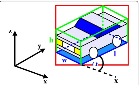
The tracking approach interacts with a 3D classification method which uses a generic parallelepiped 3D model of the expected objects in the scene. According to the best possible associations for previously tracked objects or test-ing a initial configuration for a new object, the tracktest-ing method sends a merged set of blobs to the 3D classification algorithm, in order to obtain the most likely 3D description of this blobs configuration, considering the expected objects in the scene. The parallelepiped model is described by its 3D dimensions (widthw, lengthl, and heighth), and orientationawith respect to the ground plane of the 3D referential of the scene, as depicted in Figure 3. For simpli-city, lateral parallelepiped planes are considered perpendi-cular to top and bottom parallelepiped planes.

The proposed parallelepiped model representation allows to quickly determine the object class associated to a moving region and to obtain a good approximation of the real 3D dimensions and position of an object in the scene. This representation tries to cope with the majority of the limitations imposed by 2D models, but being general enough to be capable of modelling a large variety of objects and still preserving high efficiency for real-world applications. Due to its 3D nature, this repre-sentation is independent from the camera view and object orientation. Its simplicity allows users to easily define new expected mobile objects. For modelling uncertainty associated to visibility of parallelepiped 3D dimensions, reliability measures have been proposed, also accounting for occlusion situations. A large variety of objects can be modelled (or, at least, enclosed) by a parallelepiped. The proposed model is defined as a par-allelepiped perpendicular to the ground plane of the analysed scene. Starting from the basis that a moving object will be detected as a 2D blob b with 2D limits (Xleft, Ybottom, Xright, Ytop), 3D dimensions can be

esti-mated based on the information given by pre-defined 3D parallelepiped models of the expected objects in the scene. These pre-defined parallelepipeds, which repre-sent an object class, are modelled with three dimensions

w, land hdescribed by a Gaussian distribution (repre-senting the probability of different 3D dimension sizes for a given object), together with a minimal and maxi-mal value for each dimension, for faster computation. Formally, an attribute model q˜, for an attributeq can be defined as:

˜

q= (Prq(μq, σq),qmin,qmax), (1)

Figure 3Example of a parallelepiped representation of an object. The figure depicts a vehicle enclosed by a 2D bounding box (coloured in red) and also by the parallelepiped representation. The base of the parallelepiped is coloured in blue and the lines projected in height are coloured in green. Note that the orientation

wherePrqis a probability distribution described by its

meanµqand its standard deviation sq, where q ~Prq

(µq,sq).qmin andqmaxrepresent the minimal and

maxi-mal values for the attributeq, respectively. Then, a pre-defined 3D parallelepiped model QC (a pre-defined model) for an object classCcan be defined as:

QC= (w,˜ ˜l,h),˜ (2)

where w_˜, ˜_l and _h˜ represent the attribute models for the 3D attributes width, length and height, respectively. The attributesw, landh have been modelled as Gaus-sian probability distributions. The objective of the classi-fication approach is to obtain the classCfor an object

O detected in the scene, which better fits with an expected object class modelQC.

A 3D parallelepiped instanceSO(found while proces-sing an image sequence) for an objectOis described by:

SO= (α, (w,Rw), (l,Rl), (h,Rh)), (3)

where a represents the parallelepiped orientation angle, defined as the angle between the direction of length 3D dimension and x axis of the world referen-tial of the scene. The orientation of an object is usually defined as its main motion direction. Therefore, the real orientation of the object can only be computed after the tracking task. Dimensions w, l and h repre-sent the 3D values for width, length and height of the parallelepiped, respectively. l is defined as the 3D dimension which direction is parallel to the orientation of the object. wis the 3D dimension which direction is perpendicular to the orientation. h is the 3D dimen-sion parallel to the z axis of the world referential of the scene. Rw, Rland Rh are 3D visual reliability

mea-sures for each dimension. These meamea-sures represent the confidence on the visibility of each dimension of the parallelepiped and are described in Section 3.2.5. This parallelepiped model has been first introduced in [45], and more deeply discussed in [8]. The dimensions of the 3D model are calculated based on the 3D posi-tion of the vertexes of the parallelepiped in the world referential of the scene. The idea of this classification approach is to find a parallelepiped bounded by the limits of the 2D blob b. For completely determining the parallelepiped instance SO, it is necessary to deter-mine the values for the orientation a in 3D scene ground, the 3D parallelepiped dimensions w, l, and h

and the four pairs (x,y) of 3D coordinates representing the base coordinates of the vertexes. Therefore, a total of 12 variables have to be determined.

Considering that the 3D parallelepiped is bounded by the 2D bounding box found on a previous segmenta-tion phase, we can use a pin-hole camera model

transform to find four linear equations between the intersection of 3D vertex points and 2D bounds. Other six equations can be derived from the fact that the parallelepiped base points form a rectangle. As there are 12 variables and 10 equations, there are two degrees of freedom for this problem. In fact, posed this way, the problem defines a complex non-linear system, as sinusoidal functions are involved. Then, the wisest decision is to consider variable a as a known para-meter. This way, the system becomes linear. But, there is still one degree of freedom. The best next choice must be a variable with known expected values, in order to be able to fix its value with a coherent quan-tity. Variablesw,landhcomply with this requirement, as a pre-defined Gaussian model for each of these vari-ables is available. The parallelepiped height hhas been arbitrarily chosen for this purpose. Therefore, the reso-lution of the system results in a set of linear relations in terms of h of the form presented in Equation (4). Just three expressions for w, l and x3 were derived

from the resolution of the system, as the other vari-ables can be determined from the 10 equations pre-viously discussed. For further details on the formulation of these equations, refer to [8].

w=Mw(α;M,b)×h+Nw(α;M, b)

l=Ml(α;M, b)×h+Nl(α;M, b)

x3=Mx3(α;M,b)×h+Nx3(α;M, b)

(4)

Therefore, considering perspective matrixM and 2D blob b = (Xleft, Ybottom, Xright, Ytop), a parallelepiped

instance S_Ofor a detected object Ocan be completely defined as a functionf:

SO=f(α,h,M, b) (5)

Equation (5) states that a parallelepiped modelOcan be determined with a function depending on parallele-piped heighth, and orientationa, 2D blob blimits, and the calibration matrixM. The visual reliability measures remain to be determined and are described below. 3.2.1 Classification method for parallelepiped model The problem of finding a parallelepiped model instance

SO for an object O, bounded by a blob b has been solved, as previously described. The obtained solution states that the parallelepiped orientation aand heighth

operation is performed for each blob on the current video frame.

PM(SO,C) =

q∈{w,l,h}

Prq(q|μq, σq) ₍₆₎

Given a perspective matrixM, object classification is performed for each blob b from the current frame as shown in Figure 4.

The presented algorithm corresponds to the basic optimisation procedure for obtaining the most likely parallelepiped given a blob as input. Several other issues have been considered in this classification approach, in order to cope with static occlusion, ambiguous solutions and objects changing postures. Next sections are dedi-cated to these issues.

3.2.2 Solving static occlusion

The problem of static occlusion occurs when a mobile object is occluded by the border of the image, or by a static object (e.g. couch, tree, desk, chair, wall and so on). In the proposed approach, static objects are manu-ally modelled as a polygon base with a projected 3D height. On the other hand, the possibility of occlusion with the border of the image just depends on the proxi-mity of a moving object to the border of the image. Then, the possibility of occurrence of this type of static occlusion can be determined based on 2D image infor-mation. To determine the possibility of occlusion by a static object present in scene is a more complicated task, as it becomes compulsory to interact with the 3D world.

In order to treat static occlusion situations, both pos-sibilities of occlusion are determined in a stage prior to calculation of the 3D parallelepiped model. In case of occlusion, projection of objects can be bigger. Then, the limit of possible blob growth for the image referential directions left, bottom, right and top are determined, according to the position and shape of the possibly occluding elements (polygons) and the maximal dimen-sions of the expected objects in the scene (given differ-ent blob sizes). For example, if a blob has been detected very near the left limit of the image frame, then the blob could be bigger to the left, so its limit to the left is really bounded by the expected objects in the scene. For

determining the possibility of occlusion by a static object, several tests are performed:

1. The 2D proximity to the static object 2D bound-ing box is evaluated,

2. if 2D proximity test is passed (object is near), the blob proximity to the 2D projection of the static object in the image plane is evaluated and

3. if the 2D projection test is also passed, the faces of the 3D polygonal shape are analysed, identifying the nearest faces to the blob. If some of these faces are hidden from the camera view, it is considered that the static object is possibly occluding the object enclosed by the blob. This process is performed in a similar way as [46].

When a possible occlusion exists, the maximal possi-ble growth for the possibly occluded blob bounds is determined. First, in order to establish an initial limit for the possible blob bounds, the largest maximum dimensions of expected objects are considered at the blob position, and those who exceed the dimensions of the analysed blob are enlarged. If all possible largest expected objects do not impose a larger bound to the blob, the hypothesis of possible occlusion is discarded. Next, the obtained limits of growth for blob bounds are adjusted for static context objects, by analysing the hid-den faces of the object polygon which possibly occlude the blob, and extending the blob, until its 3D ground projection collides the first hidden polygon face.

Finally, for each object class, the calculation of occluded parallelepipeds is performed by taking several starting points for extended blob bounds which repre-sent the most likely configurations for a given expected object class. Configurations which pass the allowed limit of growth are immediately discarded and the remaining blob bound configurations are optimised locally with respect to the probability measure PM, defined in Equa-tion (6), using the same algorithm presented in Figure 4. Notice that the definition of a general limit of growth for all possible occlusions for a blob allows to achieve an independence between the kind of static occlusion and the resolution of the static occlusion problem, obtaining the parallelepipeds describing the static object and border occlusion situations in the same way. 3.2.3 Solving ambiguity of solutions

As the determination of a parallelepiped to be associated to a blob has been considered as an optimisation pro-blem of geometric features, several solutions can some-times be likely, leading to undesirable solutions far from the visual reality. A typical example is the one presented in Figure 5, where two solutions are very likely geome-trically given the model, but the most likely from the expected model has the wrong orientation.

For eachclassCof pre-defined models

For allvalid pairs(h,α)

SO←F(α,h,M,b);

ifPM(SO,C)improves best currentfitS(OC)forC,

thenupdate optimalS(_OC)forC;

Class(b) =argmaxC(PM(S(OC),C));

A good way for discriminating between ambiguous situations is to return to moving pixel level. A simple solution is to store the most likely found parallelepiped configurations and to select the instance which better fits with the moving pixels found in the blob, instead of just choosing the most likely configuration. This way, a moving pixel analysis is associated to the most likely parallelepiped instances by sampling the pixels enclosed by the blob and analysing if they fit the parallelepiped model instance. The sampling process is performed at a low pixel rate, adjusting this pixel rate to a pre-defined interval of sampled pixels number. True positives (TP), false positives (FP), true negatives (TN) and false nega-tives (FN) are counted, considering a TP as a moving pixel which is inside the 2D image projection of the par-allelepiped, a FP as a moving pixel outside the parallele-piped projection, a TN as a background pixel outside the parallelepiped projection and a FN as a background pixel inside the parallelepiped projection. Then, the cho-sen parallelepiped will be the one with higher TP + TN value.

Another type of ambiguity is related to the fact that a blob can be represented by different classes. Even if nor-mally the probability measure PM (Equation (6)) will be able to discriminate which is the most likely object type, it exists also the possibility that visual evidence arising from overlapping objects give good PM values for bigger class models. This situation is normal as visual evidence can correspond to more than one mobile object hypoth-esis at the same time. The classification approach gives as output the most likely configuration, but it also stores the best result for each object class. This way, the deci-sion on which object hypotheses are the real ones can be postponed to the object tracking task, where tem-poral coherence information can be utilised in order to chose the correct model for the detected object.

3.2.4 Coping with changing postures

Even if a parallelepiped is not the best suited representa-tion for an object changing postures, it can be used for this purpose by modelling the postures of interest of an object. The way of representing these objects is to first define a general parallelepiped model enclosing every posture of interest for the object class, which can be uti-lised for discarding the object class for blobs too small or too big to contain it. Then, specific models for each posture of interest can be modelled, in the same way as the other modelled object classes. Then, these posture representations can be treated as any other object model. Each of these posture models are classified and the most likely posture information is associated to the object class. At the same time, the information for every analysed posture is stored in order to have the possibi-lity of evaluating the coherence in time of an object changing postures by the tracking phase.

With all these previous considerations, the classifica-tion task has shown a good processing time perfor-mance. Several tests have been performed in a computer Intel Pentium IV, Xeon 3.0 GHz. These tests have been shown a performance of nearly 70 blobs/s, for four pre-defined object models, a precision foraofπ/40 radians and a precision for hof 4 cm. These results are good considering that, in practice, classification is guided by tracking, achieving performances over 160 blobs/s. 3.2.5 Dimensional reliability measures

A reliability measureRqfor a dimension qÎ {w, l,h} is

intended to quantify the visual evidence for the esti-mated dimension, by visually analysing how much of the dimension can be seen from the camera point of view. The chosen function is Rq(SO) ® 0[1], where visual reliability of the attribute is 0 if the attribute is not visi-ble and 1 if is completely visivisi-ble. These measures repre-sent visual reliability as the maximal magnitude of projection of a 3D dimension onto the image plane, in proportion with the magnitude of each 2D blob limiting segment. Thus, the maximal value 1 is achieved if the image projection of a 3D dimension has the same mag-nitude compared with one of the 2D blob segments. The function is defined in Equation (7).

Ra= min

dYa·Yocc

H +

dXa·Xocc

W , 1

, (7)

where astands for the concerned 3D dimension (l, w

or h).dXaanddYarepresent the length in pixels of the

projection of the dimensionaon the XandYreference axes of the image plane, respectively. HandW are the 2D height and width of the currently analysed 2D blob.

Yocc and Xocc are occlusion flags, which value is 0 if

occlusion exists with respect to the Y orX reference axes of the image plane, respectively. The occlusion

(a) (b)

flags are used to eliminate the contribution to the value of the function of the projections in each 2D image reference axis in case of occlusion, as dimension is not visually reliable due to occlusion. An exception occurs in the case of a top view of an object, where reliability for h dimension isRh = 0, because the dimension is

occluded by the object itself.

These reliability measures are later used in the object tracking phase of the approach to weight the contribu-tion of new attribute informacontribu-tion.

3.3 Reliability multi-hypothesis tracking algorithm In this section, the new tracking algorithm, Reliability Multi-Hypothesis Tracking (RMHT), is described in detail. In general terms, this method presents similar ideas in the structure for creating, generating and elimi-nating mobile object hypotheses compared to the MHT methods presented in Section 2. The main differences from these methods are induced by the object represen-tation utilised for tracking, the dynamics model incor-porating reliability measures and the fact that this representation differs from the point representation (rather than region) frequently utilised in the MHT methods. The utilisation of region-based representations implies that several visual evidences could be associated to a mobile object (object parts). This consideration implies the conception of new methods for creation and update of object hypotheses.

3.3.1 Hypothesis representation

In the context of tracking, a hypothesis corresponds to a set of mobile objects representing a possible configura-tion, given previously estimated object attributes (e.g. width, length, velocity) and new incoming visual evi-dence (blobs at current frame). The representation of the tracking information corresponds to a hypothesis set list as seen in Figure 6. Each related hypothesis set in the hypothesis set list represents a set of hypotheses exclusive between them, representing different alterna-tives for mobiles configurations temporally or visually related. Each hypothesis set can be treated as a different tracking sub-problem, as one of the ways of controlling the combinatorial explosion of mobile hypotheses. Each hypothesis has associated a likelihood measure, as seen in equation (8).

PH=

i∈(H)

pi·Ti, ₍₈₎

whereΩ(H) corresponds to the set of mobiles repre-sented in hypothesisH,pito the likelihood measure for

a mobilei (obtained from the dynamics model (Section 3.4) in Equation (19)), and Ti to a temporal reliability

measure for a mobile i relative to hypothesisH, based on the life-time of the object in the scene. Then, the

likelihood measure PH for an hypothesisHcorresponds

to the summation of the likelihood measures for each mobile object, weighted by a temporal reliability mea-sure for each mobile, accounting for the life-time of each mobile. This reliability measure allows to give higher likelihood to hypotheses containing objects vali-dated for more time in the scene and is defined in equa-tion (9).

Ti=

Fi

j∈(H)Fj

, ₍₉₎

whereFiis the number of frames since an object i has

been seen for the first time. Then, this temporal mea-sure lies between 0 and 1 too, as it is normalised by the sum of the number of frames of all the objects in hypothesisH.

3.3.2 Reliability tracking algorithm

The complete object tracking process is depicted in Fig-ure 7. First, a hypothesis preparation phase is per-formed:

- It starts with a pre-merge task, which performs preliminary merge operations over blobs presenting highly unlikely initial features, reducing the number of blobs to be processed by the tracking procedure. This pre-merge process consist in first ordering blobs by proximity to the camera, and then merging blobs in this order, until minimal expected object model sizes are achieved. See Section 3.2, for further details on the expected object models.

frame. This set of blob potential correspondences associated to a mobile object is defined as the involved blob set which consists of the blobs that can be part of the visual evidence for the mobile in the current analysed frame. The involved blob sets allow to easily implement classical screening techni-ques, as described in Section 2.

- Finally, partial worlds (hypothesis sets) are merged if the objects at each hypothesis set are sharing a common set of involved blobs (visual evidence). This way, new object configurations are produced based on this shared visual evidence, which form a new hypothesis set.

Then, a hypothesis updating phase is performed:

on optimising the processing time performance. In this process, different visual evidence sets are merged according to expected mobile size and posi-tion, and initially merged based on the models of the expected objects in the scene.

- Then, the obtained sets of most likely tracks are combined in order to obtain the most likely hypoth-eses representing the current alternatives for a par-tial world. The hypothesis generation process is oriented on looking for the most likely valid combi-nations, according to the observed visual evidence. - After, new mobiles are initialised with the visual evidence not used by a given hypothesis, but utilised by other hypotheses sharing the same partial world. This way, all the hypotheses are complete in the sense that they provide a coherent description of the partial world they represent.

- In a similar way, visual evidence not related to any of the currently existing partial worlds is utilised to form new partial worlds according to the proximity of this new visual evidence.

A last phase of hypothesis reorganisation is then per-formed:

- First, mobiles definitely lost, and unlikely or redun-dant hypotheses are filtered (pruning process). - Finally, a partial world can be separated, when the mobile objects in it are not currently related. This process reduces the number of generated hypoth-eses, as less mobile object configurations must be evaluated.

The most likely hypotheses are utilised to generate the list of most likely mobile objects which corresponds to the output of the tracking process.

3.3.3 3D classification and RMHT interactions

The best mobile tracks and hypothesis generation tasks interact with the 3D classification approach described in Section 3.2 in order to associate the 3D information for the most likely expected object classes associated to the mobiles. As reliability of mobile object attributes increases in time (becomes stable), the parallelepiped classification process can also be guided to boost the search of most likely parallelepiped configurations. This can be done by using the expected values of reliable 3D mobile attributes to give a starting point in the search of parallelepiped attributes, and optimising in a local neighbourhood ofaandhparallelepiped attributes.

When a mobile object has validated its existence dur-ing several frames, even a better performance can be obtained by the 3D classification process, as the paralle-lepiped can be estimated just for one object class,

assuming that the correct guess has been validated. In the other extreme, when information is still unreliable to perform 3D classification, only 2D mobile attributes are updated, as a way to avoid unnecessary computation of bad quality tentative mobiles.

3.4 Dynamics model

The dynamics model is the process of computing and updating the attributes of a mobile object, considering pre-vious information and current observations. Each mobile object in a hypothesis is represented as a set of statistics inferred from visual evidences of their presence in the scene. These visual evidences are stored in a short-term history buffer of blobs representing these evidences, called blob buffer. In the case of the proposed object model com-bining 2D blob and 3D parallelepiped features, the attri-butes considered for the calculation of the mobile statistics belong to the setA= {X,Y,W,H,xp,yp,w,l,h,a}. (X,Y) is

the centroid position of the blob,WandHare the 2D blob width and height, respectively. (xp,yp) is the centroid posi-tion of the 3D parallelepiped base.w,landhcorrespond to the 3D width, length and height of the parallelepiped. At the same time, an attributeVafor each attributeaÎAis

calculated, representing the instant speed based on values estimated from visual evidence available in the blob buffer. When the possibility of erroneous and lost data is consid-ered, it is necessary to consider a blob buffer which can serve as backup information, as instant speed requires at least two available data instances.

3.4.1 Modelling uncertainty with reliability measures Uncertainty on data can arise from many different sources. For instance, these sources can be the object model, the geometry of the scene, segmentation quality, temporal coherence, appearance, occlusion, among others. Then, the design object dynamics must consider several measures for modelling these different sources. Following this idea, the proposed dynamics model inte-grates several reliability measures, representing different uncertainty sources.

- Let RVak be the visual reliability of the attribute a, extracted from the visual evidence observed at frame k. The visual reliability differs according to the attribute.

- For the 3D attributesw,landh, they are obtained with the Equation (7).

- For 3D attributesxp,ypanda, their visual

reliabil-ity is calculated as the mean between the visual reliability ofwandl, because the calculation of these three attributes is related to the base of the parallele-piped 3D representation.

camera is calculated, accounting for the fact that the segmentation error increases when objects are farther from the camera.

- When no 3D model is found given a blob, the reliability measures for 3D attributes are set to 0. This allows to restrict the incorporation of attribute information to the dynamics model, if some attribute value is lost on the current frame.

- To account for the coherence of values obtained for attribute a throughout time, the coherence relia-bility measureRCa(tc), updated to current timetc, is

defined:

RCa(tc) = 1.0−min

1.0, σa(tc)

amax−amin

, (10)

where valuesamaxandamin in (10) correspond to

pre-defined minimal and maximal values fora, respectively. The standard deviation sa(tc) of the attribute a at time

tc(incremental form) is defined as:

σa(tc) =

RV(a)·

σa(tp)2+

RVac·(ac− ¯a−(tp)) 2

RVacca(tc)

,(11)

where ac is the value of attribute a extracted from

visual evidence at frame c, andā(tp)(as later defined in

Equation (16)) is the mean value ofa, considering infor-mation until previous framep.

RVacca(tc) =RVac+e−λ·

(tc−tp)·_{RVacca(tp), (12)} is the accumulated visual reliability, adding current reliability RVac to previously accumulated valuesRVacca

(tp) weighted by a cooling function, and

RV(a) = e

−λ·(tc−tp)·_RVacca(tp)

RVacca(tc) (13)

is defined as the ratio between current and previous accumulated visual reliability, weighted by a cooling function.

The value _e−λ·(tc−tp), present in Equations (11) and (12), and later in Equation (16), corresponds to the cool-ing function of the previously observed attribute values. It can be interpreted as a forgetting factor for reinfor-cing the information obtained from newer visual evi-dence. The parameter l ≥ 0 is used to control the strength of the forgetting factor. A value of l= 0 repre-sents a perfect memory, as forgetting factor value is always 1, regardless the time difference between frames, and it is used for attributesw,l andhwhen the mobile is classified with a rigid model (i.e. a model of an object with only one posture (e.g. a car)).

Then, the mean visual reliability measure RVa(tk)

represents the mean of visual reliability measures RVa

until frame k, and is defined using the accumulated visual reliability (Equation (12)) as

RVa(tc) = RVacca(tc)

sumCooling(tc), (14)

with

sumCooling(tc) =sumCooling(tp) +e−λ·(tc−tP), (15)

wheresumCooling(tc) is the accumulated sum of

cool-ing function values.

In the same way, reliability measures can be calculated for the speed Va of attribute a. Let Vak correspond to current instant velocity, extracted from the values of attribute a observed at video frames k and j, where j

corresponds to the nearest valid previous frame index to k. Then, RVVak corresponds to the visual reliability of the current instant velocity and is calculated as the mean between the visual reliabilities RVakand RVaj. 3.4.2 Mathematical formulation of dynamics

The statistics associated to an attributeaÎ A, similarly to the presented reliability measures, are calculated incrementally in order to have a better processing time performance, conforming a new dynamics model for tracked object attributes. This dynamics model proposes a new way of utilising reliability measures to weight the contribution of the new information provided by the visual evidence at the current image frame. The model also incorporates a cooling function utilised as a forget-ting factor for reinforcing the information obtained from newer visual evidence. Considering tc as the

time-stamp of the current frame cand tpthe time-stamp of

the previous frame p, the obtained statistics for each mobile are now described.

The mean valueāfor attributeais defined as:

¯

a(tc) = ac·RVac+e−λ·

(tc−tp)·_aexp(tp)·_RVacca(tp)

RVacca(tc) ,(16)

where the expected value aexp corresponds to the

expected value for attribute aat current timetc, based

on previous information. This formulation is intention-ally related to respective prediction and filtering esti-mates of Kalman filters [22]. This computation radically differs from the literature by incorporating reliability measures and a cooling function to control pertinence of attribute data. ac is the value and RVac is the visual reliability of the attribute a, extracted from the visual evidence observed at framec.RVacca(tk) is the

Equation (12). e−λ·(tc−tP) is the cooling function. This way,ā(tc) value is updated by adding the value of the

attribute for the current visual evidence, weighted by the visual reliability for this attribute value, while pre-viously obtained estimation is weighted by the forgetting factor and by the accumulated visual reliability.

The expected valueaexpofacorresponds to the value

of a predictively obtained from the dynamics model. Given the mean valueā(tp) for aat the previous frame

timetp, and the estimated speedVa(tp) ofaat previous

framep, it is defined as

aexp(tc) =a¯(tp) +Va(tp)·(tc−tp). (17)

Va(tp) corresponds to the estimated velocity of a

(Equation (18)) at previous framep.

The statistics considered for velocity Vafollow the

same idea of the previously defined equations for attri-bute a, with the difference that no expected value for the velocity ofais calculated, obtaining the value of the statistics ofVadirectly from the visual evidence data.

The velocityVaofais then defined as

Va(tc) = Vac·RVVac +e−λ·

(tc−tp)·_Va(tp)·_RVaccV a(tp)

RVaccVa(tc)

,(18)

where Vak corresponds to current instant velocity, extracted from the aattribute values observed at video frameskandj, wherejcorresponds to the nearest pre-vious valid frame index prepre-vious tok. RVV_ak corresponds

to the visual reliability of the current instant velocity as defined in previous Section 3.4.1. Then, visual and coherence reliability measures for attribute Vacan be

calculated in the same way as for any other attribute, as described in Section 3.4.1.

Finally, the likelihood measure pm for a mobilemcan

be defined in many ways by combining the present attri-bute statistics. The chosen likelihood measure forpmis

a weighted mean of probability measures for different groups of attributes ({w, l, h} as D3D, {x, y} as V3D, {W,

L} as D2D, and {X,Y} as V2D), weighted by a joint

relia-bility measure for each group, as presented in Equation (19).

pm= k∈K

RkCk k∈KRk

(19)

withK= {D3D,V3D,D2D,V2D} and

CD3D =

d∈{w,l,h}(RCd+Pd)RVd

2

d∈{w,l,h}

RDd

(20)

CV3D=

MPV+PV+RCV

3.0 , (21)

CD2D =Rvalid2D·

RCW+RCH

2 , (22)

CV2D=Rvalid2D·

RCVX+RCVY

2.0 , (23)

where Rvalid2D is the Rvalid measure for 2D informa-tion, corresponding to the number of not lost blobs in the blob buffer, over the current blob buffer size.

From Equation (19):

-RD2D =Rva1id2D

RVW(tc)+RVH(tc)

2

with RVW(tc) and RVH(tc) mean visual reliabilities of

WandH, respectively.

-RV2D =Rva1id2D

RVX(tc)+RVY(tc)

2

with RVX(tc) and RVY(tc) mean visual reliabilities of

Xand Y, respectively.

-RD3D =Rva1id3D

RVw(tc)+RV1(tc)+RVh(tc)

3

with RVw(tc), RV1(tc), and RVh(tc) the mean visual

reliabilities for 3D dimensions w, land h, respectively.

Rvalid3D corresponds to the number of classified blobs in the blob buffer, over the current blob buffer size.

- RV3D=Rva1id3D

RVx(tc)+RVy(tc)

2

with RVx(tc), and RVy(tc) the mean visual reliabilities

for 3D position coordinatesx, andy, respectively. Measures CD2D, CD3D, CV2D, and CV3D are considered as measures of temporal coherence (i.e. discrepancy between estimated and measured values). The measures

RV3D, RV3D, RD2D and RV2D are the accumulation of visi-bility measures in time (with decreasing factor).Pw,Pl

andPhin Equation (20) correspond to the mean

prob-ability of the dimensional attributes according to the a priori models of objects expected in the scene, consider-ing the coolconsider-ing function as in Equation (16). Note that parameter tchas been removed for simplicity. MPV, PV

and RCVvalues present in Equation (21) are inferred

from attribute speeds Vx and Vy. MPVrepresents the

probability of the current velocity magnitude

V =V2

object model, and defined in the same way as other attribute models described in Section 3.2. PV

corre-sponds to the mean probability for the position prob-abilities PVx and PVy, calculated with the values of Pw and Pl, as the 3D position is inferred from the base

dimensions of the parallelepiped.RCVcorresponds to

the mean between RCVx and RCVy. This way, the value

pmfor a mobile objectmwill mostly consider the

prob-ability values for attribute groups with higher reliprob-ability, using the values that can be trusted the most. At the same time, different aspects of uncertainty have been considered in order to better represent and identify sev-eral issues present in video analysis.

4 Evaluation and results

In order to validate the approach, two tests have been performed. The objective of the first test is to evaluate the performance of the proposed tracking approach in terms of quality of solutions. against the participants of the ETISEO project [47] for video analysis performance evaluation benchmarking. The obtained results have been compared with algorithms developed by 15 anon-ymous participants in the ETISEO project, considering four benchmark videos publicly available, which are part of the evaluation framework. The objective of the sec-ond test is to evaluate the performance of the proposed tracking approach in terms of quality of solutions and time performance, suppressing different features of the proposed approach, against a known tracker implemen-tation. For this purpose, the performance of the pro-posed approach has been compared with the OpenCV frame-to-frame tracker [42] implementation, presented in Section 2. The same videos of the ETISEO project have been used for this test, considering versions with only 2D features and suppressing the reliability effect, in order to understand the contribution of each feature of the approach. Also a single-object video has been tested to give a closer insight of the effects of multi-target to object associations (poorly segmented objects). The tests were performed with a computer with processor Intel Xeon CPU 3.00 GHz, with 2 Giga Bytes of memory. For obtaining the 3D model information, two parallelepiped models have been pre-defined for person and vehicle classes. The precision on 3D parallelepiped height values to search the classification solutions has been fixed in 0.08 (m), while the precision on orientation angle has been fixed inπ/40(rad).

4.1 Test I: Quality test against ETISEO participants For evaluating the object tracking quality of the approach, the Tracking Time metric (TTrackedfrom now

on), utilised in ETISEO project, has been considered. This metric measures the ratio of time that an object

present in the reference data has been observed and tracked with a consistent ID over tracking period. The match between a reference datum RD and a physical object Cis done with the bounding box distance D1 and with the constraint that object ID is constant over the time. The distance value D1 is defined in the con-text of ETISEO project as the dice coefficient, as twice the overlapping area between RD and C, divided by the sum of both the area ofRDand C(Equation (24)).

D1 = 2·area(RD∩C)

area(RD) +area(C) (24)

This matching process can give as result more than one candidate object Cto be associated to a reference objectRD. The chosen Ccandidate corresponds to the one with the greatest intersection time interval with the reference objectRD. Then, the tracking time metric cor-responds to the mean time during which a reference object is well tracked, as defined in Equation (25).

TTracked= 1

NBRefData

RefData

card(RD∩C)

card(RD) , (25)

where the functioncard() corresponds to the cardinal-ity in terms of frames. From the available videos of the ETISEO project, the videos for evaluating the TTracked

metric are:

- AP-11-C4: Airport video of an apron (AP) with one person and four vehicles moving in the scene over 804 frames.

- AP-11-C7: Airport video of an apron (AP) with five vehicles moving in the scene over 804 frames. - RD-6-C7: Video of a road (RD) with approximately 10 persons and 15 vehicles moving in the scene over 1200 frames.

- BE-19-C1: Video of a building entrance (BE) with three persons and one vehicle over 1025 frames.

In terms of the Tracking Time metric, the results are summarised in Figure 8. The results are very competi-tive with respect to the other tracking approaches. For this experiment, 15 of the 22 participants of the real evaluation cycle have presented results for the Tracking Time metricb. Over these tracking results, the proposed approach has the second best result on the apron videos, and the third best result for the road video. The worst result for the proposed tracking approach has been obtained for the building entrance video, with a fifth position. In terms of reconfiguration between videos, the effort was minimal.

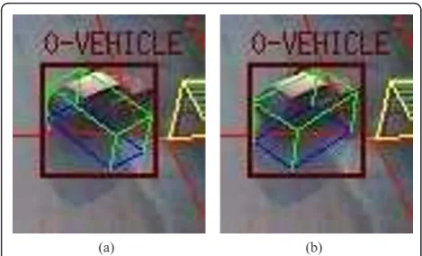
bounding box enclosing an object means that the cur-rently associated blob has been classified, while a red one means that the blob has not been classified. The white bounding box enclosing a mobile corresponds to its 2D representation, while yellow lines correspond to its 3D parallelepiped representation. Red lines following the mobiles correspond to the 3D central points of the parallelepiped base found during the tracking process for the object. In the same way, blue lines following the mobiles correspond to the 2D representation centroids found.

- AP-11-C4: For the first apron video, a Time Track-ing metric value of 0.68 has been obtained. Accord-ing to the appearance of the obtained results, it seemed that the metric value would be higher, as apparently no track has been lost over the analysis of the video. The metric value could have been affected by parts of the video where tracked objects became totally occluded until the end of the sequence. In this case, the tracking approach dis-carded these paths after certain number of frames.

Results of the tracking process for this video are shown in Figure 9.

- AP-11-C7: For the second apron video, a Time Tracking metric value of 0.69 has been obtained. Similarly to the first video sequence, a higher metric value was expected, as apparently no track had been lost over the analysis of the video. The metric value could have been affected by the same reasons of video AP-11-C4. Results of the tracking process for this video are shown in Figure 10.

- RD-6-C7: For the road video, a Time Tracking metric value of 0.50 has been obtained. This video was hard compared with the apron videos. The main difficulties of this video were the total static occlu-sion situations at the bottom of the scene. At this position, the objects were often lost, because they were poorly segmented, and when the static occlu-sion situation occurred, no enough reliable informa-tion was available to keep their track, until they reappeared in the scene. Nevertheless, several objects were appropriately tracked and even the lost objects by static occlusion were correctly tracked after the 0

0.1 0.2 0.3 0.4 0.5 0.6 0.7 0.8 0.9 1

G1 G3 G8 G9 G12 G13 G14 G15 G17 G19 G20 G23 G28 G29 G32 MZ

Tracking Time Metric

Research Group

AP-11-C4 AP-11-C7 RD-6-C7 BE-19-C1

Figure 8Summary of results for the Tracking Time metricTTrackedfor the four analysed videos. The labels starting with aG, at the

problem, showing a correct overall behaviour of the tracking approach. This video presented a real chal-lenge for real-time processing as often nearly ten objects were tracked simultaneously. Results of the tracking process for this video are shown in Figure 11. A video with the tracking results is also publicly availablec.

- BE-19-C1: For the building entrance video, a Time Tracking metric value of 0.26 has been obtained. This video was the hardest of the four analysed videos, as presented dynamic occlusion situations and poor segmentation of the persons moving in the scene. Results of the tracking process for this video are shown in Figure 12.

The processing time performance of the proposed tracking approach has been also analysed in this experiment. Unfortunately, ETISEO project has not incorporated the processing time performance as one of its evaluation metrics, thus it is not possible to

compare the obtained results with the other tracking approaches. Table 1 summarises the obtained results for time metrics: mean processing time per frame Tp,

mean frame rate Fp, standard deviation of the

proces-sing time per frame σTp and maximal processing time utilised in a frame T_p(max). The results show a high pro-cessing time performance, even for the road video RD-6-C7 (Fp= 42.7(frames

s)), which concentrated sev-eral objects simultaneously moving in the scene. The fastest processing times for videos AP-11-C7 (Fp= 85.5(frames

s)) and BE-19-C1

(Fp= 86.1(frames

s)) are explained from the fact that there was a part of the video where no object was pre-sent in the scene, and because of the reduced number of objects. The high performance for the video AP-11-C4 (Fp= 76.4(frames

the Tp and σTp metrics show that this maximal value can correspond to isolated cases.

4.2 Test II: Testing different features of the approach For this test, different algorithms are compared in order to understand the contribution of the different features:

- Tracker2D-R: A version of the proposed approach, suppressing 3D features.

- Tracker2D-NR: A version of the proposed approach, suppressing 3D features and reliability measures effect (every reliability measure set to 1). - OpenCV-Tracker: The implementation of the OpenCV frame-to-frame tracker [42].

First, tests have been performed using the four ETI-SEO videos utilised in Section 4.1, evaluating the

TTracked metric and the execution time performance.

Tables 2 and 3 summariseTTrackedmetric and execution

time performance, respectively. The videos of the results for Tracker2D-R, Tracker2D-NR and Tracker-OpenCV

algorithms are available online at http://profesores.elo. utfsm.cl/~mzuniga/video.

According to theTTrackedmetric, the results show that

the quality of tracking is greatly improved considering 3D features (see Table 2), and slightly improved consid-ering reliability measures with only 2D features. It is worthy to highlight that the 3D features compulsory need the utilisation of reliability measures for represent-ing not found 3D representations, occlusion and lost frames, among other issues. Even if utilising or not the reliability measures for only 2D features does not make a high difference in terms of quality, more complicated Figure 11Tracking results for the road video RD-6-C7.

Figure 12Tracking results for the building entrance video BE-19-C1.

Table 1 Evaluation of results obtained for both analysed video clips in terms of processing time performance.

Video Length Fp(frames/s) Tp(s) σTp(s) Tp(max)(s)

AP-11-C4 804 76.4 0.013 0.013 0.17

AP-11-C7 804 85.5 0.012 0.027 0.29

RD-6-C7 1200 42.7 0.023 0.045 0.56

BE-19-C1 1025 86.1 0.012 0.014 0.15

scenes result in a better time performance when using reliability measures, as can be noticed in the time per-formance results for sequences RD6-C7 and BE19-C1, at Table 3. The Tracker3D highly outperforms OpenCV-Tracker in quality of solutions, obtaining these results with a higher time performance. Both Tracker2D ver-sions outperform the quality performance of OpenCV-Tracker, while having a better time performance in almost an order of magnitude. Finally, in order to illus-trate the difference in performance considering the multi-target to object association capability of the pro-posed approach, we have tested the Tracker2D-R ver-sion of the approach versus the OpenCV-Tracker on a single-object sequence of a rodentd. Figure 13 shows an illustration of the obtained sequence. The complete sequence is available online at http://profesores.elo. utfsm.cl/~mzuniga/video/VAT-HAMSTER.mp4. The sequences clearly show the smoothness achieved by the proposed approach in terms of object attributes estima-tion, compared with OpenCV-Tracker. This can be jus-tified with the robustness of the dynamics model given by the cooling function, reliability measures and proper generation of multi-target to object hypotheses.

4.3 Discussion of results

The comparative analysis of the tracking approach has shown that the proposed algorithm can achieve a high performance in terms of quality of solutions for video scenes of moderated complexity. The results obtained by the algorithm are encouraging as they were always over the 69% of the total of research groups and out-performed OpenCV-Tracker both in time and quality performance. It is important to consider that no sys-tem parameter reconfiguration has been made between different tested videos, as one of the advantages on

utilising a generic object model. In terms of processing time performance, with a mean frame rate of 70.4 (frames/s) and a frame rate of 42.7(frames/s) for the hardest video in terms of processing, it can be con-cluded that the proposed object tracking approach can have a real-time performance for video scenes of mod-erated complexity when 3D features are utilised, while the time performance using only 2D features is consid-erably higher, showing also a good quality/time compromise.

The road and building entrance videos have shown that there are still unsolved issues. Both road and build-ing entrance videos show the need of new efforts on the resolution of harder static and dynamic occlusion pro-blems. The interaction between the proposed parallele-piped model with appearance models can be an interesting first approach to analyse in the future for these cases. Nevertheless, appearance models are not useful in case of noisy data, bad contrast or objects too far in the scene, but the general object model utilised in the proposed approach, together with a proper manage-ment of possible hypotheses, allows to better respond to these situations.

5 Conclusion

Addressing real-world applications implies that a video analysis approach must be able to properly handle the information extracted from noisy videos. This require-ment has been considered by proposing a generic mechanism to measure in a consistent way the reliability of the information in the whole video analysis process. More concretely, reliability measures associated to the object attributes have been proposed in order to mea-sure the quality and coherence of this information. The proposed tracking method presents similar ideas in the structure for creating, generating and eliminating mobile object hypotheses compared to the MHT methods. The main differences from these methods are induced by the object representation utilised for tracking and the fact that this representation differs from the point represen-tation normally utilised in the MHT methods. The utili-sation of a representation different from a point representation implies the consideration of the possibi-lity that several visual evidences could be associated to a mobile object. This consideration implies the conception

Table 2 Quality evaluation using TTrackedmetric, for different versions of the proposed approach and the OpenCV-Tracker.

Tracker AP11-C4 AP11-C7 BE19-C1 RD6-C7

Tracker3D 0.68 0.69 0.26 0.50 Tracker2D-R 0.49 0.69 0.17 0.47 Tracker2D-NR 0.49 0.67 0.16 0.47 OpenCV-Tracker 0.41 0.65 0.12 0.48

Table 3 Time performance evaluation for different versions of the proposed approach and the OpenCV-Tracker.

Tracker AP11-C4 AP11-C7 BE19-C1 RD6-C7 Total Mean

(frame/s) μ(s) (frame/s) μ(s) (frame/s) μ(s) (frame/s) μ(s) (frame/s) μ(s)