ECE-320 Labs 7 and 8:
Utilizing a dsPIC30F6015 to control the speed of a wheel
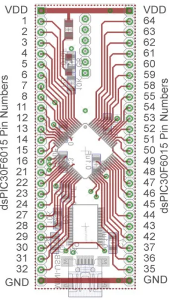
Overview: In this lab we will utilize the dsPIC30F6015 to implement a PID controller to control the speed of a wheel. Most of the initial code will be given to you (see the class website), and you will have to modify the code as you go on. One of the things you will discover is that you often need to be aware of limitations of both hardware and software when you try to implement a controller. The dsPIC30F6015 has been mounted on a carrier board that allows us to communicate with a terminal (your laptop) via a USB cable. In what follows you will need to make reference to the pin out of the dsPIC30F6015 (shown in Figure 1) and the corresponding pins on the carrier (shown in Figure 2)
Part A (Copying the initial files)
Set up a new folder for this lab, and copy the files for this Lab from the class website to this folder.
Part B (Downloading and installing MPLAB)
You will need to go to the website
http://www.microchip.com/stellent/idcplg?
IdcService=SS_GET_PAGE&nodeId=1406&dDocName=en019469
and download the newest version of MPLAB (MPLAB IDE v8.83+). If you have an older of MPLAB it will probably work (mine is v8.76) and you may be able to skip this step. It is probably easiest to download a zipped version and the unzip it. Once the file has been unzipped, run setup.exe. Accept all of the defaults. Do not intall any C compilers yet.
Part C (Downloading and installing MPLAB C30 compiler)
You will need to go to the website
http://www.microchip.com/stellent/idcplg?
IdcService=SS_GET_PAGE&nodeId=1406&dDocName=en536656
and download the MPLAB C compiler for the dsPIC. This is the academic version. You will need to register your use (click on register now). Once the file has been downloaded, you need to run
mplab30_v3_30c_windows.exe to install it. I used the Versioned Directory Name. Select the
Evaluation Compiler. The devices we want are the dsPIC DCSs Part D (Setting up Communications with Secure CRT)
In this step we will make sure all of our systems are working before we go on.
Connect the PICkit3 to the carrier board and your computer (the white arrow goes near the white spot on the carrier board.)
Connect the separate communication cable to the carrieer board and your computer.
Connect power to the power board and toggle to on switch (the green LED should then be on)
We are going to want to be able to record and plot data, so we will be writing to the screen. In order to do this we will using Secure CRT because it is installed on your computer by default.
Go to ProgramsAll ProgramsSecureCRTSecureCRT6.2 (it’s ok if you don’t have 6.2). You should get a screen like this (although the list of Sessions will probably be shorter for you):
You should then get a screen that looks like this
Click on New Session
Choose Serial
from this menu, then click on Next
You will next get the following screen. You should already know which port to use (it may not be COM5 on your computer). Select a Baud rate of 115200 and be sure everything is filled in as below. The click on Next.
Finally, you will get a screen like that below, and you need to select Connect.
Now you should have a terminal like that shown below
Part E (Putting it all together)
Now we are ready to start. Note that at some point in the following process you may need to let the system download firmware. Be sure you have selected the correct device (or it will do this twice).
Start MPLAB
Select Project and open the project lab7.mcp
Select Configure, then Select Device and choose dsPIC30F6015
Select Debugger, then Select Tool and choose PICkit 3
You may need to clickon lab7.c (under Source Files) to see the C code. You should get a screen (more or less) like the following:
You should compile the existing program, download it to the dsPIC, and run it. You should see a sequence of numbers on your screen (the secure CRT screen). These correspond to sample times.
Download (to dsPIC) Run
Part F (Turning one LED on and off)
In this step we will make one LED turn on and off.
Locate pin 1 (RE5). Connect a resistor and an LED to this pin as shown below:
We need to get this ready for output, so in the file lab7.c, insert the lines (before the main loop) TRISEbits.TRISE5 = 0;
You will see in the main loop we are writing all 1’s or all zeros to all of port E every other time interval.
Compile your code and run it. Your LED should turn on and off regularly.
Part G (Running Two LEDs)
Connect your other LED to pin2 (RE6). Modify you code so the LED’s alternate (one goes on and the other off). Once this has been checked off (see the last page) , comment out the code that turns the LEDs on and off in the main code (do not delete it).
Have this verified by your instructor.
Part H (Utilizing PWM to run your LEDs)
We will now utilize the PWM function to drive the LED. Note that RE6 corresponds to PWM4L.(Refer to Figures 1 and 2 to be sure to get the correct pin. Note that not all of the dsPIC pins are on the carrier.) In the routine pwm_init, change PWM_PDIS4L to PWM_PEN4L. This allows us to use this pin as a PWM signal. In the main code, uncomment the function call pwm_init();
Uncomment the code:
dutycycle = (unsigned int) ((double) AD_value)*scale; dutycyclereg = 4;
SetDCMCPWM( dutycyclereg, dutycycle, updatedisable);
This code determines the duty cycle value and writes it to dutycycle register 4.
Compile and run your code. A single LED should light (constantly).
Modify the values in AD_value from 0 to 512 to verify that the brightness of the LEDs changes as the dutycycle changes. Note that at some point the LED stops getting brighter, so don’t worry about that. Have the instructor verify this (see the last page).
Part I (Reading in an A/D value)
Now we want to be able to connect a potentiometer so we can have a variable reference. The software is currently set up for A/D input on AN3/RB3. You will need to do the following things:
1) Connect the potentiometer as shown below 2) Set the appropriate TRIS bits for an input signal
3) Comment out the part of the code that sets the AD_value = 0;
4) Modify the printf statement to allow you to also print out the A/D value from the pot
Have this verified by your instructor (see the last page).
Part K: Reading in the sensor transducer
In order to determine how fast the motor is spinning, we will need to use the QEI interface. The sensor is connected to the center of the wheel, and the other end of the sensor plugs into the breadboard. The pins for the interface are shown in Figure 3. You need to connect this interface to +5 volts (red ), ground (blue), and the QEA Channel A input (pin 12), and the QEA Channel B input (pin 11).
Figure 3. Encoder pin outs.
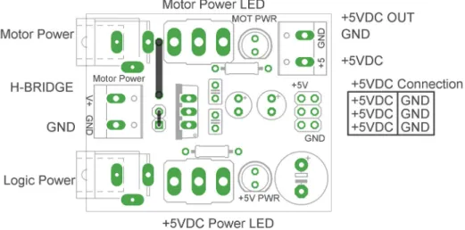
Part L: Connecting the power entry
Plug in both the 5 volt (green) and 12 volt (red) power supplies, as shown in Figure 4. Do not turn on the supplies yet (the LEDs should be off) .
Part M: Connecting the H Bridge
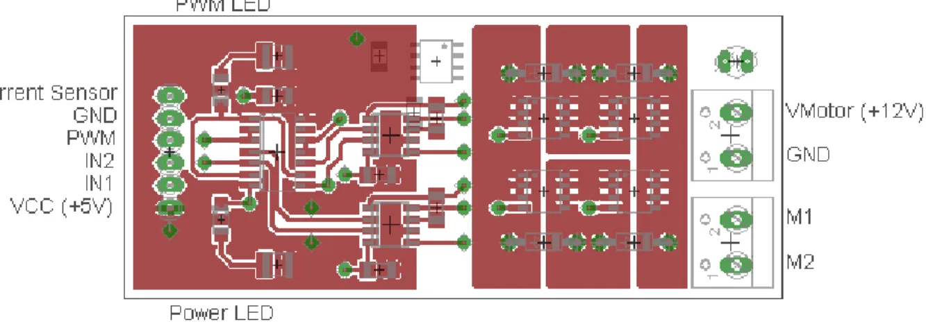
Plug in the H-bridge, shown in Figure 5. You are going to need access to the different pins, so be sure it is located in a place you can easily get wires to.
Figure 5. H Bridge connections
Starting on the left, connect the ground and +5 volt supplies. Next, connect IN1 to E6 (pin 2) and IN2 to E7 (pin 3). (Note that if the motor speed is negative you may want to reverse these connections.) Finally connect PWM to PWM 3 high (pin 1).
Starting on the right, connect (with the twisted wires) the 12 volt power from the power entry module to the 12 volt input. Be sure to connect ground to ground and +12 to +12. Next, connect M1 and M2 (using the twisted wires) to the motor input.
At this point all of your wiring should be done. You should check it over before you go on. Two important things to keep in mind as you do the remainder of this lab:
Use the red switch to shut off power to the motor. Sometimes stopping the dsPIC does not stop the motor, in which case you will need to use the switch.
Unless you are told otherwise (and later in the lab you will be), turn the pot fairly slowly.
PART N: Determining Initial Scaling
steady value (it will likely keep getting faster). Do this for three different positions of the pot where the steady state speed is less than 150 rad/sec.
We now want to determine the proportionality constant between the A/D value read from the pot and the motor speed in rad/sec. Compute the three scaling factors and average them (mine was approximately 0.31).
Change the parameter AD_scale (in your code) to this value. Run the system again at various input values. It may take a while for the system to reach steady state. Compare your reference input to the actual output. They should be fairly close for speeds below 100 rad/sec, but they will not be exact.
PART O: Proportional Control
We now want to start with our first control scheme, proportional control. You will need to declare the variable kp as a double (at the top of the main routine). Outside of the main loop set kp = 1.0, and inside the main loop, after both the speed and reference input are determined, compute the error as error = R-speed. Here R is the reference input and speed is the measured output speed of the wheel in
rad/sec. The control effort is then proportional to this error, so u = kp *error.
Recompile and download the code onto the microcontroller. Now start the system again. Move the pot to a number of different set points, and wait until the system comes to steady state. Most likely the steady state value will be approximately one half of the set point.
Stop the system and change the value of kp to 5, and then to 10. (Be sure to recompile and download after each time). Run the system again for each value of kp. You should notice that the steady state error gets smaller each time.
PART P: Limiting the slope of the control effort
One of the first limitations we will have to deal with is the fact that if you try and draw too much power all at once, the power supply assumes you have screwed up. This leads to some strange behavior.
Starring with kp = 10.0, start the system and turn the pot (setting the reference input) as quickly as you can (but don’t worry about turning it all the way). Mostly likely you hear strange sounds from the motor like it is starting and stopping (or worse).
insure that the value of u is within acceptable limits. Finally, you will need to set the value for
MAX_DELTA_U. I would start at around 800, and change this as necessary. Try to get this value as large as possible. Run your code and try to change the pot (the reference input) as quickly as possible. Once you think your values are ok, set kp=100.0 and be sure your system runs acceptably (the motor does not shut off and on).
PART Q: Proportional controllers with large gains
Make sure kp is set to 100 for this part. Compile the code if you need to and start it running. Vary the reference signal to a few set points (such as 30 rad/sec, 60 rad/sec, and 90 rad/sec) and allow the system to try and reach steady state at each of these set points. You should notice that as the set point increases in value, the speed of the wheel starts to vary significantly from the reference point. Part of this is due to the fact that the motor is only capable of one direction, but a larger part is due to the fact that small errors are amplified (by 100) and this causes the motor to continually oscillate.
PART R: Integral control
Recall that using a prefilter to control steady state error can sometimes be problematic since the prefilter is outside the feedback loop. An alternative, and generally better, solution is to include some form of integral control. Recall that an integral controller has the form
Rearranging this we get
In the time-domain this becomes
Since we want the control effort as our output, we will write this as
Hence to implement the integral control, we need to sum the error terms and then scale them by .
Declare two new (double) variables Isum and ki. Set the initial value of Isum to zero outside the main loop. Within the main loop update the error summation using something like Isum = Isum + error.
Within the main loop implement a PI controller as follows:
u = kp*error + ki*Isum;
Set kp = 0.0 and ki = 0.5. Modify the print statement at the end of your code so the value of Isum is also printed out. Recompile and download your code. Start the system and set the reference signal to a few reference points (30, 60, 90 rad/sec, for example), and let the system run for a while. Your system will probably exhibit some pretty strange behavior on its way to the correct steady state value (it will bounce around the steady state value due to sampling). Look at what is happening to the value of Isum during this strange behavior.
PART S: Integrator problems
The first problem we need to fix is that our motor is only spinning in one direction. When Isum
becomes large and negative, we would expect the motor to spin in the other direction, but it can’t. One way to minimize this effect is to check to be sure that the value of Isum is greater than or equal to zero. Modify your code to do this, recompile, and run it again.
The second problem we have is called integrator windup. Basically, the accumulated error is becoming too large and causes the system to overshoot, and then undershoot. One way to fix this is to limit the value of Isum to a maximum value. There is a defined variable at the beginning of the code
MAX_ISUM. You need to set a reasonable value for this variable and limit the value of Isum be less than this max. Modify your code to do this, recompile, download, and run it again. You will have to use some trial and error to find a good value for MAX_ISUM since it is also a function of the value of ki. I choose a value somewhere between 10 and 800 (I’m not telling you where, but I am suggesting
someplace to start looking). Do not move on until you have what you think is a reasonable value of
PART T: Including a derivative term
Finally we need to include a derivative term to implement a full PID controller. You will need to define three new (double) variables, kd, Derror, and last_error. Outside of the main loop set Derror and
last_error equal to zero and set kd equal to 0.01. Inside the main loop include the lines
Derror = error-last-error; Last_error = error;
Finally, to implement the full PID controller define the control error u to be
u = kp*error+ki*Isum+kd*Derror;
Compile and download your code, and try a few reference points. Your system may still oscillate, but we can work on that soon.
PART U: Designing a PID controller
At this point, we want to hardcode the value of the reference signal so the step response will start as soon as we turn on the system. Just after the statement where we assign R based on the A/D value, insert the statement
R = 90.0; // set for 90 rad/sec
A general plan for designing a PID controller using a trial and error method (we have no model for the plant) is the following:
First, set ki = kd = 0, and try to get a good response for a step input using only kp.
Next, adjust ki to get a good steady state error. Since the integral control tends to slow the system down, don’t make this any larger than you need to. However, you may need to also change MAX_ISUM to get a good response.
Finally, adjust kd to speed up the response.
Once you have a good design, you need to log your data so you can make a Matlab plot. If you have saved your data in a file named (for example) play3.log, then in Matlab type
Design PID controllers to meet the specifications shown below. Include a Matlab generated figure of your step response results in your memo, and be sure to include both the sampling interval and the values of kp, ki, and kd. Also attach your final code to your e-mail.
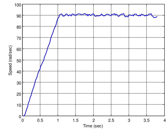
(i) For a sampling interval of T = 0.025 sec (the default) our design criteria is a settling time of less than or equal to 1.2 seconds, and a percent overshoot less than 10%.
(ii) For a sampling time of 0.1 sec, our design criteria is a settling time of less than or equal to 4.0 seconds, and a percent overshoot less than 10%.
(iii) For a sampling time of 0.1 sec, design a PID controller so there is at least a 10% overshoot and the settling time is less than 10 seconds.
0 0.5 1 1.5 2 2.5 3 3.5 4
0 10 20 30 40 50 60 70 80 90 100 S pe ed (r ad /s ec ) Time (sec)
Figure 6: Step response for system with T = 0.025 seconds. I am not telling you my parameter values.