Volume 2008, Article ID 716826,14pages doi:10.1155/2008/716826
Review Article
Antenna Subset Selection for Cyclic Prefix Assisted MIMO
Wireless Communications over Frequency Selective Channels
A. Wilzeck1and T. Kaiser2
1Institute of Communications Technology, Leibniz University of Hannover, Appelstr. 9a, 30167 Hannover, Germany 2mimoOn GmbH, Technology Center of Duisburg, Bismarckstr. 120, 47057 Duisburg, Germany
Correspondence should be addressed to A. Wilzeck,[email protected]
Received 31 May 2007; Revised 21 September 2007; Accepted 15 January 2008
Recommended by Markus Rupp
Antenna (subset) selection techniques are feasible to reduce the hardware complexity of multiple-input multiple-output (MIMO) systems, while keeping the benefits of higher-order MIMO systems. Many studies of antenna selection schemes are based on frequency-flat channel models, which are inconsistent to broadband MIMO systems employing spatial-multiplexing. In broadband MIMO systems aiming to provide high-data-rate links, the employed signal bandwidth is typically larger than the coherence bandwidth of the channel so that the channel will be of frequency selective nature. Within this contribution we provide an overview on joint transmitter- and receiver-side antenna subset selection methods for frequency selective channels and deploy them in MIMO orthogonal frequency division multiplexing (OFDM) systems and MIMO single-carrier (SC) systems employing frequency domain equalization (FDE).
Copyright © 2008 A. Wilzeck and T. Kaiser. This is an open access article distributed under the Creative Commons Attribution License, which permits unrestricted use, distribution, and reproduction in any medium, provided the original work is properly cited.
1. INTRODUCTION
The use of multiple antennas at receiver- and/or transmitter-side, that is, the so-called multiple-input multiple-output (MIMO) systems is nowadays an almost mandatory part of today’s and emerging wireless communications standards (e.g., IEEE 802.11n, WiMax, 3GPP long term evolution (LTE)). They enable high data rates, enhanced link quality or range extension, and interference mitigation techniques without requiring additional precious resources such as bandwidth or transmission power. The utilization of all these benefits of the MIMO technology is unfortunately not possible to its full extent at the same time, but MIMO enables—beside the time, frequency, and code domain— another degree of freedom: the spatial domain. Thus, sophisticated and advanced algorithms are required to utilize all domains in different communication scenarios yielding to a rich set of trade-offs.
In high data-rate communications, a signal bandwidth that is higher than the channel coherence bandwidth is typically employed, so frequency selective fading degrades the performance of a communication link. Two signaling schemes with reasonable complexity of equalization are
Nevertheless, the spatial domain, as an additional degree of freedom, comes at the expense of extra analogue and digital hardware, creating additional costs, power con-sumption, and space requirements. Therefore, the use of multiple antennas is challenging and requires a smart system and antenna design especially in mobile devices. Antenna (subset) selection techniques at receiver- and/or transmitter-side can help to relax the complexity burden of a higher-order MIMO system, while preserving some of its benefits in a MIMO system of lower order. A limited feedback is required from the receiver to the transmitter in order to perform the selection of the transmit antenna subsets if the use of the frequency division duplex (FDD) mode is assumed, where uplink and downlink communications are considered to be done in different frequency bands, spaced far apart from each other. In time division duplex (TDD) mode, the transmitter might be able to gather the required channel knowledge via its uplink, but exploiting the channel reciprocity might become questionable in practice due to radio frequency (RF) front-end mismatches [5].
Antenna (subset) selection schemes for MIMO wireless communications are an active research area and draw a lot of attention from information theory and practice. Here, we aim to highlight some related and relevant publications of the recent years. A study on the ergodic capacity for receive and transmit antenna selection in a flat fading channel can be found in [6]. In [7], spatial multiplexing in flat fading channels employing transmit antenna selection and linear receivers is studied. A vertical Bell labs layered space time (V-BLAST) type detection in conjunction with transmit antenna selection in a MIMO communication system is given in [8]. Receive antenna subset selection with successive interference cancellation (SIC) and linear minimum mean square error (MMSE) receivers with joint encoding of data streams are discussed in [9]. The challenge of fast subset antenna selection is studied in [10]. Receive antenna subset selection for correlated flat fading MIMO channels is treated in [11, 12]. A comparison between beam selection and antenna selection techniques for indoor MIMO systems is provided in [13]. Recently, a study on the performance of systems employing linear receivers and receive antenna selection under the presence of cochannel interference was published in [14]. A MIMO OFDM system with transmit antenna selection criteria for a frequency selective fading channel can be found in [15]. Implementation aspects and the effects of nonideal hardware on MIMO antenna selection schemes can be found in [16], and in [17] more explicitly for the IEEE 802.11n specification. Main challenges are the channel training design for antenna selection schemes, insertion loss caused by additional RF components (e.g., RF switches), and RF mismatches requiring a selection-dependent calibration. The performance of maximum likelihood (ML) receivers in an MIMO OFDM system with transmit antenna selection based on channel state information (CSI) feedback is studied in [18]. Joint transmit- and receive antenna selection with capacity maximizing algorithms is given in [19], whereas extensive overviews on the research in the area of antenna (subset) selection schemes can be found in [20, 21]. A practical eigenbeam MIMO OFDM testbed employing
trans-mit antenna selection is studied in [22], where it is shown that a “2 out of 3” transmit antenna scheme reaches the performance of a system with 3 transmit antennas. It is further reported that a significant better performance than an eigenbeam-only system with 2 transmit antennas can be achieved. Studies employing antenna selection schemes in spacetime-coded MIMO systems can be found in [23–26], but the discussion on spacetime coding is out of the scope of this contribution, as we consider systems employing spatial multiplexing.
The rest of this contribution is organized as follows. An overview on the signaling schemes for MIMO OFDM and MIMO SC-FDE is given inSection 2. Here, a common system model for both schemes is defined and extended towards antenna subset selection at transmitter and receiver side. In addition, the requirements regarding the limited feedback from the transmitter to the receiver are discussed. In Section 3, a compilation of antenna (subset) selection metrics for frequency selective channels is given. Beside this, each selection method is also discussed concerning its implementation requirements. InSection 4, the average bit error rate (BER) performance of MIMO OFDM and MIMO SC-FDE systems employing the different antenna subset selection methods is compared. The deployed channel model can be seen as a typical benchmark channel model for MIMO communications over frequency selective channels. A first comparison is done based on an uncoded 2(3)×2(3) MIMO SC-FDE system employing a linear zero forcing (ZF) or MMSE equalizer, where the number in brackets within the MIMO system configuration indicates the number of available antennas. In addition, the antenna subset selection methods employing convolutional encoded 2(3) × 2(3) MIMO SC-FDE and MIMO OFDM systems are compared. A simulation result with noisy channel knowledge is further given to emphasize the challenge to quickly acquire a high-quality estimate of the different antenna subset channels. Section 5concludes this contribution.
2. SYSTEM MODEL
In this section, we first introduce the MIMO OFDM and the MIMO SC-FDE schemes with the help of a common framework, with the further addition of antenna subset selection at the transmitter and receiver side to the system model.
Note that such systems would have nearly the same 3 dB transmit signal bandwidth, but the steepness of the slope of the power spectral density (PSD) is quite important for fitting to a given spectral mask. The roll-off factor is an important design parameter—especially for the synchroniza-tion in time—and influences directly the steepness of the slope of the PSD and the occupied bandwidth. SC-based systems usually utilize higher roll-offfactors for their pulse shaping filters than OFDM-based ones. Nevertheless, for both systems it is possible to fulfill such a mask without loss of spectral efficiency [2], but this happens only when the system parameters are well chosen. A realistic comparison of MIMO OFDM and MIMO SC-FDE taking such parameters and requirements into account can be found in [27].
Under the assumption of perfect synchronization in time and frequency, the pulse-shaping filters and corresponding matched filters can be included into the channel. Hence, the discrete-time baseband transmit signal for a single block transmission duration of a MIMO OFDM system can be given as
sOFDM=
Es
NT
INT⊗
PaddF−N1
d, (1)
where Iz is the z ×z identity matrix; the operator “⊗”
indicates the Kronecker product;FN is theN ×N Fourier
matrix with elements [FN]n,μ = (1/ √
N)exp(−j2π(nμ/N)), where n = {0, 1,. . .,N −1} is the sample number and μ= {0, 1,. . .,N−1}is the frequency tone number.Paddis
a matrix adding a cyclic prefix (CP) of lengthPto a block of lengthN. The (N+P)×NmatrixPaddis defined as
Padd=
⎛
⎝0P×(N−P) IP
IN
⎞
⎠, (2)
where0indicates a zero matrix of a given size. TheNNT×1 vectord =[dT1,dT2,. . .,dTNT]
Tdescribes in
parallel transmitted data blocks dnT = [d0,d1,. . .,dN−1]
T,
each consisting ofN consecutive M-PSK (PSK: phase-shift keying) orM-QAM (QAM: quadrature amplitude modula-tion) symbols. The notation [·]T means the transpose of a
matrix or vector. The factor Es/NTensures that the MIMO
transmitter radiates the same overall transmit power as a single-input single-output (SISO) system.Es is the symbol
energy. In an OFDM system, the inverse Fourier matrixF−N1
is employed to modulate the data-block dnT of the nTth transmit antenna onNsubcarriers.
From (1), the transmit signal of a MIMO SC-FDE system can be obtained by multiplying each dnT with the Fourier matrixFN,
sSCFDE=
Es
NT
INT⊗
PaddF−N1FN
d, = Es NT
INT⊗Padd
d.
(3)
Thereby, the inverse Fourier matrixF−1
N is eliminated.
Here, two interesting points can be noticed:
(1) SC-FDE can be seen as a special case of an OFDM sys-tem, where some kind of nonredundant “precoding” of the data blocks with the help of the Fourier matrix FNis employed;
(2) due to this “precoding,” SC-FDE directly exploits frequency diversity. The entire time-domain data symbol is spread over theNsubcarriers. In contrast to this, OFDM directly uses time diversity. Nevertheless, both schemes need channel coding in order to obtain diversity from the domain not directly used.
The received signal of both systems is given as
r=Hlins+ν, (4)
where r = [rT1,r2T,. . .,rTNR]
T is an (N +P)N
R ×1 vector,
which contains the received signal of theNRreceive antennas,
s = [sT
1,sT2,. . .,sTNT]
T is a (N +P)N
T ×1 vector, which
contains the transmit signals of the NT transmit antennas
corresponding to (1) or (3), andν = [νT
1,νT2,. . .,νTNR]
T is a
(N+P)NR×1 vector, which contains the complex Gaussian
noise—independent and identically distributed (i.i.d.) with zero mean—added at each of theNRreceive antennas.
Hlin is defined as a block matrix, containing all linear
channel matricesHnR,nTbetween thenTth transmit and the nRth receive antenna,
Hlin=
⎛ ⎜ ⎜ ⎜ ⎜ ⎜ ⎜ ⎜ ⎝
H1,1 H1,2 . . . H1,NT
H2,1 H2,2 . . . H2,NT ..
. ... ... ...
HNR,1 HNR,2 . . . HNR,NT
⎞ ⎟ ⎟ ⎟ ⎟ ⎟ ⎟ ⎟ ⎠ . (5)
We define the (N+P)×(N+P) linear channel matrix (discrete-time linear convolution matrix) as
HnR,nT=
⎛ ⎜ ⎜ ⎜ ⎜ ⎜ ⎜ ⎜ ⎜ ⎜ ⎜ ⎜ ⎜ ⎜ ⎜ ⎜ ⎜ ⎜ ⎜ ⎜ ⎜ ⎜ ⎜ ⎜ ⎜ ⎝
h0;nR,nT 0 . . . 0 h1;nR,nT h0;nR,nT . . . 0
h2;nR,nT h1;nR,nT . . . 0 ..
. ... . . . ...
h(L−1);nR,nT h(L−2);nR,nT . . . h0;nR,nT
0 h(L−1);nR,nT . . . h1;nR,nT
0 0 . . . h2;nR,nT ..
. ... . . . ...
0 0 . . . h(L−1);nR,nT
⎞ ⎟ ⎟ ⎟ ⎟ ⎟ ⎟ ⎟ ⎟ ⎟ ⎟ ⎟ ⎟ ⎟ ⎟ ⎟ ⎟ ⎟ ⎟ ⎟ ⎟ ⎟ ⎟ ⎟ ⎟ ⎠ , (6)
where hl;nR,nT is the lth complex discrete-time baseband channel coefficient (with l = {0, 1, 2,. . .,L−1}) between thenTth transmit and thenRth receive antenna, andLis the
Transmitter De-m ultiple xer βd OFDM SC-FDE d1 d2
dNT
s1
s2
sNT
ν1
ν2
νNR r1
r2
rNR
˘r1
˘r2
˘rNR Hlin
F−1 N
F−1 N
F−1 N IN IN IN . . . Padd Padd Padd Prem Prem Prem . . . FN FN FN W IN IN IN . . .
F−1 N
F−1 N
F−N1 d1
d2
dNT
M ultiple xer d Receiver
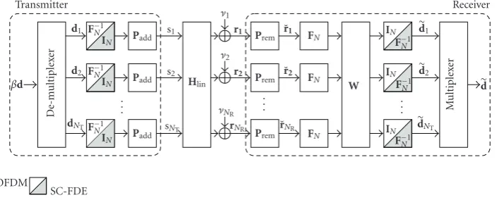
Figure1: Joint block diagram of spatially multiplexed MIMO OFDM and MIMO SC-FDE systems,β= Es/NT.
The first task in both systems is the removal of the CP on each of theNRreceived signals, which usually requires at least
a coarse synchronization. The signal after CP removal is
˘
r=INR⊗Prem
r, (7)
where
Prem=
0N×P IN
(8)
performs the CP removal and is of sizeN×(N+P). The addition of a CP at transmitter side and the removal of the CP at receiver side converts all linear channel matrices (elements of block channel matrix Hlin) into circulant
channel matrices,
Hc=
INR⊗Prem
Hlin
INT⊗Padd
. (9)
The received signal after passing the circulant channel matrix can be given as
˘
r=Hc˘s+ ˘ν, (10)
where ˘s is the transmit signal before adding the CP, ˘ν = (INR ⊗Prem)ν, and ˘r is the received signal after removing the CP. Since only samples are removed from ν, the type of the distribution of the noise in ˘νis not changed, but the autocorrelation of the noise is affected by the convolution with a rectangular window.
In the case of MIMO OFDM, the equalized received data can then be given as
dOFDM=WDFN,NRHcDF−1
N,NT
Es
NT
d+WDFN,NRν˘, (11)
whereDZ,z =Iz⊗Zis a block diagonal matrix withztimes
the matrixZas elements, andWis a MIMO equalizer matrix. Due to the fact that a circulant channel matrix can be diagonalized by right-hand multiplication withF−N1and
left-hand multiplication withFN, we obtain that the matrix
Λ=DFN,NRHcDF−1
N,NT (12)
is a block diagonal matrix.
The block elements are [Λ]nR,nT = diagonal(FNhnR,nT), wherehnR,nT =[h0;nR,nT,h1;nR,nT,. . .,hL−1;nR,nT, 0,. . ., 0]Tis an N ×1 vector containing the discrete-time linear channel impulse response between the nTth transmit antenna and
nRth receive antenna.
We now can rewrite (11) as
dOFDM=WΛ
Es
NT
d+WDFN,NRν.˘ (13)
A similar result can be obtained for MIMO SC-FDE
dSCFDE
=DF−1
N,NRWDFN,NRHcDF−N1,NTDFN,NT
Es
NT
d+DF−1
N,NRWDFN,NRν˘
=DF−1
N,NRWΛDFN,NT
Es
NT
d+DF−1
N,NRWDFN,NRν.˘
(14)
Compared to the MIMO OFDM system, it becomes obvious that the Fourier matrices inDFN,NT perform some kind of “precoding,” while the “decoding” at receiver side is performed by DF−1
N,NR for MIMO SC-FDE. In addition, the inverse Fourier matrix in DF−1
N,NR is unitary, so it will distribute the colored noise onto the resulting time-domain symbols of a receiver branch. Per time-domain symbol, this can be seen as a noise averaging process [2]. Nevertheless, this would not reduce the overall noise power included in a single block as the inverse Fourier matrix is unitary.
Figure 1 provides a joint view of the overall system model. It is worth mentioning that only in this mathematical formulation the complexity of SC-FDE seems doubled. As shown in Figure 1, the inverse Fourier matrix deployed at the transmitter side is just moved to the receiver side. In conclusion, MIMO OFDM and MIMO SC-FDE show overall the same system complexity.
Considering spatially uncorrelated MIMO channels, the linear MIMO MMSE equalizer matrixWMMSEcan be written
for both systems identically as
WMMSE=
NT
Es
ΛH
ΛΛH+NTσ
2
ν Es
INNR
†
Tx digital signal processing
DAC DAC
DAC RF 1 RF 2
RFKT
. . .
Antenna subset selection
KT
out of NT
1 2
NT
. . .
1 2
NR
. . .
Antenna subset selection
KR
out of NR
RF 1 RF 2
RFKR
. . .
ADC ADC
ADC
Rx digital signal processing
Rx-to-Tx feedback
Figure2: Antenna subset selection on transmit side (Tx) and receiver side (Rx).
where (·)† denotes the pseudo-inverse, (·)H indicates the
hermitian transpose operation, andσ2
ν represents the noise
power. Settingσ2
ν = 0, one can obtain the linear zero forcing
(ZF) equalizer as
WZF=
NT
Es
ΛHΛΛH†=
NT
Es
Λ†. (16)
Now, we assume a MIMO system that hasNT transmit
antennas and NR receive antennas, but with only KT <
NT transmit radio frequency (RF) modules and KR < NR
receive RF modules being used as shown inFigure 2. Then, the system model is reduced to aKR×KT MIMO system.
Therefore, the dimensions of vectors and matrices are from now on changed accordingly.
In case of antenna subset selection one has
BT=
⎛ ⎝NT
KT
⎞
⎠= NT!
KT!
NT−KT
!, (17)
possible selections at the transmitter side, and
BR=
⎛ ⎝NR
KR
⎞
⎠= NR!
KR!
NR−KR
!, (18)
possible selections at the receiver side. From this we can conclude that we haveB=BTBRpossible selections.
Therefore, theNKR×NKT block channel matrix H(linb)
is a subset of Hlin, where b indicates the selected subset
combination.
In order to include antenna (subset) selection in our system model, we only have to modify (13) and (14) to
d(OFDMb) =W(b)Λ(b)
Es
KT
d+W(b)D FN,KRν˘
(b),
d(SCFDEb) =DF−1
N,KRW
(b)Λ(b)D FN,KT
Es
KT
d
+DF−1
N,KRW
(b)D FN,KRν˘
(b).
(19)
A general drawback of antenna (subset) selection is that the channel knowledge can not be obtained at the same time so that a more or less opportunistic search over all possible
subset combinations is required to acquire the channel knowledge, and to select the antenna subset combination with the highest benefits for the link. Additionally, this search enhances also the risk that the selection is performed based on outdated channel knowledge, especially when the channel varies rapidly with time. Hence, it motivates the employment of fast antenna selection algorithms as given in [9,10].
As shown in Figure 2, a limited feedback is required from the receiver to the transmitter in order to perform the selection of the transmit antenna subset. Such a feedback, for example, given as channel quality indicator (CQI) and MIMO mode indicator (MMI), is currently embedded in most wireless communication standards but is usually limited to 4–6 bits per frame. For a direct selection of the subsetsNbit=log2(BT), bits are required.
In TDD mode, it might be also possible to perform the transmit antenna selection without a feedback, as the transmitter might be able to acquire the channel knowledge on its own uplink. The usage of channel reciprocity is questionable in practical systems because RF front-end effects cannot be neglected. Therefore, a calibration of the RF front-end [5] is required, which itself is depending on the selected antennas.
If the switching order of the antenna subsets is predefined (e.g., a list), the feedback can be limited further to a single bit, where “1” would mean switching to the next antenna subset on the list and “0” would indicate to keep the current subset at transmitter side, while the receiver might switch between itsBRsubsets to find the optimum antenna subset. A
two-directional access to such a list would require three states (2 bits), which would be already enough to directly access all transmitter subsets in the cases whereKT=2,NT=3,KT=
3, andNT=4.
Methods for feedback bit reduction in antenna selection schemes are studied in [28]. These reduction methods become necessary especially for systems with a higher number of possible selections or when the number of bits per frame available for feedback is quite limited.
3. SELECTION METRICS
3.1. Selection based on channel capacity optimization (CCO) methods
0 2 4 6 8 10 12 14 16
A
chie
ved
ergodic
C
(bps/Hz)
0 2 4 6 8 10 12 14 16 18 20 SNR (dB)
L=1:Cmax
L=1:Cmin
L=1: fixed
L=4:Cmax
L=4:Cmin
L=4: fixed (a) Channel LengthL= {1, 4}
0 2 4 6 8 10 12 14 16
A
chie
ved
ergodic
C
(bps/Hz)
0 2 4 6 8 10 12 14 16 18 20 SNR (dB)
L=1:Cmax
L=1:Cmin
L=1: fixed
L=15:Cmax
L=15:Cmin
L=15: fixed (b) Channel LengthL= {1, 15}
Figure3: Ergodic capacity of a 2(3)×2(3) MIMO system.
channel capacity. Since we assume that the transmitter has no knowledge about the actual frequency responses of the channels, we distribute the total transmit power PT =
E{sHs} in equal shares among the activated K
T transmit
antennas. The antenna subset selection allows the access to Bdifferent MIMO channels so that the channel capacity— or more exactly the mutual information—under the subset combinationbcan be described by
C(b)= 1
N N−1
μ=0
log2det
IKR+ ρ KT
Λ(b,μ)Λ(b,μ)H
= 1 N
N−1
μ=0
C(b,μ),
(20)
whereμis an index to the frequency tone, andρ=PT/σν2˘is an
average SNR defined here as the ratio of total transmit power PTand the noise power after removal of the cyclic prefix.
The subcarrier MIMO channel matrixΛ(b,μ)is given as
Λ(b,μ)=
⎛ ⎜ ⎜ ⎜ ⎜ ⎝
Λ(b)ξ(μ,1),ξ(μ,1) . . . Λ(b)ξ(μ,1),ξ(μ,KT) ..
. ... ...
Λ(b)ξ(μ,KR),ξ(μ,1) . . . Λ(b)ξ(μ,KR),ξ(μ,KT)
⎞ ⎟ ⎟ ⎟ ⎟ ⎠,
(21)
where ξ(μ,x) = μ+ 1 +N(x −1). The matrix Λ(b) = DF,KRH
(b)
c D−F,1KT is a block matrixwith elements [Λ
(b)]
q,p =
diagonal(FNh(qb,)p), whereh(qb,p)is anN×1 vector containing the
linear channel impulse response between the pth transmit antenna and qth receive antenna of the corresponding selectionb.
The subcarrier channel capacityC(b,μ) can be
reformu-lated as
C(b,μ)=log2det
IKR+ ρ KT
Λ(b,μ)Λ(b,μ)H
,
= q(b,μ)
i=1
log2
1 + ρ KTλ
(b,μ)
i
,
(22)
whereq(b,μ)=rank(Λ(b,μ)) is the rank of the subcarrier
chan-nel matrix andλ(ib,μ)is theith eigenvalue ofΛ(b,μ)(Λ(b,μ))Hfor
theμth frequency tone under antenna subset selectionb. With the help of (20), it is possible to perform the antenna subset selection in such a way that always the MIMO channel under which theinstantaneous channel capacityC(b)
of the MIMO channel achieves its maximum over all possible configurations. Due to the block processing structure of MIMO OFDM and SC-FDE,bhas to be selected at least for a transmission interval of a single block or more practically for a frame duration.
Taking (20) into consideration, an exhaustive search overBpossible configurations and computationally complex calculations based on the acquired channel knowledge are required to find the optimum antenna subset combinationb in terms of channel capacity. Hence, it motivates for applying incremental and decremental methods as described in [9, 10] for frequency-flat channels. Nevertheless, the exhaustive search over all possible configurations provides an upper bound of the maximum channel capacity achievable via selection.
It is claimed in [20,21], for the case of frequency selective channels, that antenna selection may not be feasible or useful because for different frequencies different antenna subsets are optimal.
with zero mean), thus yielding to a blockwise static Rayleigh fading channel. The power of each channel impulse response is normalized to 1, in order to have a strict definition of the SNR at the receiver.
The curve forCmax refers to the selection where always
the antenna sets are chosen which have a maximum instan-taneous channel capacity, whereasCminrefers to the selection
where always the antennas sets are chosen which provide a minimum instantaneous channel capacity. As a reference curve, the ergodic channel capacity for a fixed selection is included, where the antennas 1 and 2 at the transmitter and receiver sides are employed. Therefore, the curve of Cmax
represents the best case and the curve ofCminthe worst case
in terms of achievable channel capacity.
At a first glance,Figure 3seems to support the aforemen-tioned claim by [20,21]. For higher channel length Lthe curves referring toCmax andCmin are getting closer to the
fixed selection. This holds true for the achieved ergodic chan-nel capacity and also for the instantaneous chanchan-nel capacity. Consider the frequency flat caseL=1, which is plotted for reference purposes in Figure 3, it is easy to notice that compared to the fixed selection the gain in theCmaxselections
is lower than the loss possible inCmin selections. Therefore,
an erroneous selection can create a high loss in channel capacity.
On the other hand,Figure 3supports also the question, whether the channel capacity is the only and/or best metric for antenna (subset) selection in frequency selective chan-nels. Since all possible antenna (subset) selections are more or less equivalent in terms of channel capacity, other criteria should be considered. This is especially valid in practical systems, where suboptimal receivers and suboptimal channel coding are often employed.
3.2. Selection based on singular values of the MIMO channel matrix
One can find in the literature two methods to select antennas based on the knowledge of the minimum and maximum singular value of the MIMO channel matrices. In this section, we will give a straightforward approach to extend these methods to frequency selective channels.
Method 1. Select the channel with the maximum minimum eigenvalue.
As shown in [7], for flat fading channels, the smallest eigenvalue ofHHH, whereHis a flat fading MIMO channel
matrix, has the highest impact to the performance of linear ZF equalizers. The nonzero eigenvalues of HHH are λ
i = σ2
i, whereσi are the nonzero singular values of the MIMO
channel matrixH.
An extension to frequency selective channels can be done by performing the selection of b by first searching for the minimum eigenvalue of the matrices (Λ(b,μ))HΛ(b,μ),
then searching for the smallest over all (Λ(b,μ))HΛ(b,μ), and
finally searching for the antenna subset combinationbIwith
the maximum minimum eigenvalue over all possible subset combinations:
bI=arg max
b
min μ mini λ
(b,μ)
i . (23)
Note thatΛ(b,μ) is of sizeKR×KT withKR ≥ KT and that
(Λ(b,μ))HΛ(b,μ)will be of sizeK
T×KT, which allows to search
overKTeigenvalues for the minimum eigenvalue.
Method 2. Select the channel with the maximum ratio of the minimum eigenvalue and the maximum eigenvalue. This metric is inspired by the proposal in [15,29], where a similar technique is employed for switching between beam forming and spatial multiplexing.
The ratio is an indication for the spread of the eigenvalues of (Λ(b,μ))HΛ(b,μ). Lower spread means higher ratio, which
means a better conditioned channel. The criterion can be expressed as
bII=arg max
b
minμminiλ(ib,μ)
maxμmaxiλ
(b,μ)
i
. (24)
An advantage of the Methods (1,2) is that they are solely based on the acquired channel knowledge and that they can be independently deployed from the equalizer. The complex-ity of Method2is slightly higher than that of Method1, as it requires the calculation of two eigenvalues and their ratios per frequency toneμand subset combinationb.
There do exist many methods for the calculation of the eigenvalues. The first choice is to use symbolic calculations of the eigenvalues of a K ×K matrix Awith the help of det(A−λI) =! 0. Calculation of the determinant results in the so-called characteristic equation, which is a polynomial of maximum Kth order. For dimensions K ≤ 3, the determinant can be directly calculated with theSarrus Rule. The resulting characteristic polynomial is then quadratic or cubic, where closed-form solutions for its roots (equivalent to the eigenvalues) can be given. Therefore, the closed-form calculation of the eigenvalues makes sense if the antenna selection is based on aKR ≤ 3 orKT ≤ 3 system. In this
case, at least one of the matrices possible for calculating the eigenvalues—(Λ(b,μ))HΛ(b,μ) or Λ(b,μ)(Λ(b,μ))H—will match
the dimension requirement. Note that two or three RF branches per device are common for IEEE 802.11n devices deployed in a wireless local area network (WLAN).
For matrices of higher dimensions, numerical methods are more suitable. These algorithms are typically iterative. A well-known one is the QR algorithm and its modifications. It allows finding iteratively all eigenvalues and eigenvectors of a matrix. The power iteration (PI) algorithm gives the maximum eigenvalue of a matrix. Correspondingly, the inverse power iteration (IPI) yields the minimum eigenvalue of a matrix. An enhanced version of PI and IPI is the Rayleigh quotient iteration (RQI) algorithm, which converges much faster than PI and IPI. An overview on eigenvalue calculation and their practical impacts can be found in [30].
In simulations presented later on we used the SVD function provided by MATLAB to obtain all singular values of the subcarrier channel matricesΛ(b,μ).
3.3. Selection based on post-equalizer signal quality
succeeding detector or decoder. Therefore, a possible selec-tion method is to choose the antenna subset combinaselec-tionb, which provides the best signal quality at the equalizer output. A typical signal quality metric is the Euclidean distance between thenth received and equalized symbol, and thenth awaited symbol (e.g., training symbol):
Δ(b)
n = dn(b)−dn. (25)
The signal to sistortion ratio (SDR) for a block of length Ncan be defined as
SDR(b)=
N−1
n=0 d (b)
n 2
N−1
n=0 d (b)
n −dn
2. (26)
SDR is also known as equalized received modulation error ratio (MER). Another related signal quality metric is the error vector magnitude (EVM).
As pointed out in [31], the major advantage of using a signal quality metric based on the equalizer output signal is that it can inherently handle all effects (e.g., synchronization errors, channel estimation errors, hardware effects, and spatial correlation) which can degrade the quality of the equalizer output signal. Thereby, it enables the receiver to directly recognize the loss of signal quality and take appropriate actions (e.g., switching to another antenna set).
In order to use such a metric, channel training sequences or pilot symbols would be passed through the equalizer, which is usually not done, though possible. The Euclidean distance is typically already calculated by some detectors and decoders-typically based on the Viterbi algorithm, so no additional hardware is required except some infrastructure. A decision oriented approach not requiring known symbols can be based on the Euclidean distance of the input and output symbol of detectors.
In the later comparison, we use blocks of length N consisting of random quadrature phase-shift keying (QPSK) symbols as training sequences and estimate the SDR at the equalizer output.
Figure 4shows the SDR metric behavior over SNR for a MIMO SC-FDE system employing a ZF equalizer. SDRmax
corresponds to the subset selections, where the subsets with the maximum instantaneous SDR are selected, and SDRmin
to the subset selections where the subsets with the minimum instantaneous SDR are selected. The different SDR curves are almost parallel to each other over SNR in dB. Interestingly, SDRmax equals to the given SNR for the flat channel (L =
1), while for the other curves the effects due to noise amplification or perfectly not perfectly invertible channel matrices become visible.
3.4. Selection based on received signal strength indication (RSSI)
The RSSI of thekRth receiver branch is typically based on the
estimation of the average received signal power. In practice, the averaging can only be done over a short-time interval, which can be the duration of a certain part of the received signal (e.g., a preamble or some training symbols). Typically,
−20 −16 −12 −8 −4 0 4 8 12 16 20
SDR
(dB)
0 2 4 6 8 10 12 14 16 18 20 SNR (dB)
L=1: SDRmax
L=1: SDRmin
L=1: fixed
L=15: SDRmax
L=15: SDRmin
L=15: fixed
Figure 4: SDR metric of a 2(3)×2(3) MIMO SC-FDE system employing a ZF equalizer, channel lengthL= {1, 15}.
such a measurement of theinstantaneous received power is performed by the RF transceiver IC to allow for an automatic gain control (AGC). An AGC per antenna branch is required in order to match the dynamic range of the received signals to the dynamic range of the analog-to-digital converter (ADC) stage of the MIMO receiver so that the resolution of the ADC is fully exploited. In most receiver architectures, the AGC is controlled by the baseband IC so that the so-called RSSI is directly accessible from the baseband processing.
An advantage of this method is that it does not require any channel knowledge to select the receive and/or transmit antennas for signaling. A possible and simple selection algorithm works under the premise to select those antenna subsets at receive side and transmit side that are maximizing the total average receive power. A general drawback is that this method is effective only for frequency-flat or very moderately frequency selective channels [20]. In addition, this method is quite sensitive to interfering signals. Since it cannot distinguish between the power of the desired signal and the power of interfering signals, this technique might prefer antenna subsets with heavy interference, even when the desired signal is very weak.
Similar selection approaches are based on the norm of the MIMO channel matrix as given in [20,21]. This norm-based approaches are not sensitive to interference but also effective only for flat or moderately frequency-selective channels.
4. COMPARISON
The comparison of the selection methods in terms of their achieved average bit error ratio (BER) performance is carried out with Monte-Carlo simulations. The selection based on the RSSI is not taken into account because it is effective only for diversity schemes and very sensitive to interference.
Table1: Channel and simulation parameters.
Simulation parameters
Total transmit power Normalized to 1 Number of realizations for
theNNR×NNTmatrixHlin
. . .for uncoded transmission 2000 . . .for coded transmission 3000
Channel update AfterQ=4 block durations (including CP)
Reselection of subsets After newEb/N0setting Channel parameters
Channel coefficients Gaussian, i.i.d. with zero mean Spatial correlation none
Mean power delay profile Equal gain Channel length L=15 symbols Channel normalization Ll=−01|hl;nR,nT|2 !=1
blocks per antenna. The purpose of adopting the quasistatic Rayleigh fading MIMO channel model is to provide a typical benchmark channel, while it is not claimed that this channel model is realistic. The channel parameters and simulation parameters are given inTable 1.
Especially, we point out that the channel impulse responses are normalized for constant energy (seeTable 1), and hence the (average) received energy does not fluctuate over the channel realizations. This corresponds to a rich scattering environment (e.g., indoor), where the received SNR is assumed to be equal for all receive antennas. Therefore, the antenna subset selection is only based on the frequency-selective nature of the channels, which is a worst case for antenna selection schemes because it excludes the case of potentially different receive SNRs. It is clear that different levels of the received SNR will yield a gain by antenna subset selection compared to a fixed selection. One might, for example, think about the following scenario: multiple-directional receive antennas steer into different directions and receive signals from a terminal, which moves, for example, on circle around the receiver. Here, clearly the received SNR will be different and dependent on the position of the transmitter.
Due to the fact that linear equalizers are of low com-plexity and high practical importance, the linear MIMO ZF and linear MIMO MMSE equalizers are deployed for the previously introduced MIMO SC-FDE and MIMO OFDM systems performing a “2 out of 3” antenna selection at the transmitter and receiver side. This means that overall 3 different antenna subsets on each side exist, yielding to 9 different combinations. The use of more antennas at transmitter or receiver side can improve the diversity gain further, especially if we would assume a different receive SNR per antenna.
It is worth mentioning here that, as shown in [32], also ML-like receivers for MIMO OFDM are nowadays imple-mentable with reasonable complexity. The performance of ML receivers in a MIMO OFDM system with transmit
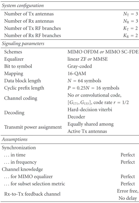
Table2: System and signaling parameters.
System configuration
Number of Tx antennas NT=3
Number of Rx antennas NR=3
Number of Tx RF branches KT=2
Number of Rx RF branches KR=2
Signaling parameters
Schemes MIMO OFDMorMIMO SC-FDE
Equalizer linear ZForMMSE Bit to symbol Gray-coded
Mapping 16-QAM
Data block length N=64 symbols Cyclic prefix length P=0.25N=16 symbols Channel coding Noorconvolutional code,
[G171,G133], code rater=1/2
Decoding Hard-decision viterbi Decoder
Transmit power assignment Equally shared among Active Tx antennas
Assumptions
Synchronization
. . .in time Perfect
. . .in frequency Perfect
Channel knowledge
. . .for MIMO equalizer Perfect
. . .for subset selection metric Perfect
Rx-to-Tx feedback channel Error free, No delay
antenna subset selection is studied in [18]. Other interesting results are given in [7] for frequency-flat channels, where a system without transmit antenna selection, but with ML receiver, was deployed as a reference system.
Table 2 gives further information about the system configuration, the signaling parameters and the assumptions used. Most of the chosen parameters are corresponding to a MIMO extended IEEE 802.11a standard and are meant as an example for benchmarking.
Figure 5 shows the uncoded BER performance of a 2(3)×2(3) MIMO SC-FDE system with linear ZF or MMSE equalizer for different settings of the channel length L. Figures5(a),5(c), and5(e)show the performance obtained by deploying a linear ZF equalizer, whereas the linear MMSE equalizer is deployed to generate Figures5(b),5(d), and5(f). FromFigure 5(a), we can see that, for the frequency-flat case, the obtained BER performance of the antenna subset selections method based on Cmax, SDRmax, the maximum
minimal eigenvalue (referred as max min EV), and based on the maximum ratio of minimum eigenvalue and maximum eigenvalue (referred as max ratio), respectively, is identical. The performance gain compared to the fixed selection is approximately 16 dB at an average BER of 10−2. Also, the
10−4
10−3
10−2
10−1
100
Av
er
ag
e
B
E
R
0 2 4 6 8 10 12 14 16 18 20 Eb/N0(dB)
(a) Linear ZF equalizer, channel lengthL=1
10−4
10−3
10−2
10−1
100
Av
er
ag
e
B
E
R
0 2 4 6 8 10 12 14 16 18 20 Eb/N0(dB)
(b) Linear MMSE equalizer, channel lengthL=1
10−4
10−3
10−2
10−1
100
Av
er
ag
e
B
E
R
0 2 4 6 8 10 12 14 16 18 20 Eb/N0(dB)
(c) Linear ZF equalizer, channel lengthL=8
10−4
10−3
10−2
10−1
100
Av
er
ag
e
B
E
R
0 2 4 6 8 10 12 14 16 18 20 Eb/N0(dB)
(d) Linear MMSE equalizer, channel lengthL=8
10−4
10−3
10−2
10−1
100
Av
er
ag
e
B
E
R
0 2 4 6 8 10 12 14 16 18 20 Eb/N0(dB)
Cmax
Cmin
SDRmax
SDRmin
Max min EV Max ratio Fixed (e) Linear ZF equalizer, channel lengthL=15
10−4
10−3
10−2
10−1
100
Av
er
ag
e
B
E
R
0 2 4 6 8 10 12 14 16 18 20 Eb/N0(dB)
Cmax
Cmin
SDRmax
SDRmin
Max min EV Max ratio Fixed (f) Linear MMSE equalizer, channel lengthL=15
onCminand SDRmin, respectively, show the same and very
poor performance.Figure 5(c)is based on a channel length ofL = 8. Here, the performance of the different selection methods starts to diverge more from each other. The best performance is obtained by the max min EV method and the max ratio method, followed by the SDRmax method,
which shows a 1 dB worse performance at a BER of 10−3.
The performance of theCmaxmethod is around 4.5 dB worse.
The fixed selection, the Cmin selection, and the SDRmin
selection show much worse performance, since the slope of the performance curve is much less steep than all other performance curves. In the case of a channel length ofL = 15,Figure 5(e)shows a similar result asFigure 5(c).
FromFigure 5(b)can be concluded that in the frequency-flat case the performance of the linear MMSE equalizer is slightly better than in the ZF case as shown inFigure 5(a). The overall ranking of the selection methods is the same. In Figure 5(d)with channel lengthL = 8, it can be observed that the curves are much closer to each other. Especially, the curves representing the fixed selection, the Cmin selection,
and the SDRminselection are now steeper than the
frequency-flat case. The performance of the Cmin and the SDRmin
selections is identical. The reason for the improvements is that the impact of noise amplification is greatly relaxed by the linear MMSE equalizer. The best performance is still obtained by the eigenvalue-based methods, max min EV, and max ratio, as they have around 3 dB better performance at a BER of 10−3 than the fixed selection, but only a marginal
advantage compared to the Cmax and SDRmax methods.
Figure 5(e)shows overall the same ranking of the methods, whereas the SDRmaxmethod and theCmaxmethod perform
similarly to each other, but marginally worse than the eigenvalue-based methods, which perform approximately 2.5 dB better compared to the fixed selection.
A quite interesting phenomenon is that the linear ZF equalizer is able to reach the performance of the linear MMSE equalizer due to some antenna subset selection schemes. The reason is that the max min EV, max ratio, and SDRmaxmethods prefer the selection of channels, which have
no or little fades in the transfer function, so the issue of noise amplification is greatly relaxed for the linear ZF equalizer.
Noticing that an OFDM-based scheme essentially requires channel coding, and/or adaptive modulation or adaptive loading of its subcarriers [2]; we consider now a convolutional encoded transmission to allow OFDM to make use of frequency diversity. The transmitted bit stream is encoded with a rate r = 1/2 convolutional encoder with generator polynomials [G171,G133] so that both transmitted
data streams are jointly encoded. The received and detected bit stream is decoded with a hard-decision Viterbi decoder. Due to the code rate, the net bit rate is reduced to half of the bit rate of the uncoded system.
Figure 6presents the average BER performance results for coded 2(3)×2(3) MIMO SC-FDE (Figures 6(a) and 6(b)) and MIMO OFDM (Figures 6(c) and 6(d)) for a channel length of L = 15. Comparing first Figures 6(a) and 6(c), where an linear ZF equalizer is deployed, we can see that the MIMO SC-FDE scheme suffers heavily from noise amplification but is able to reach a performance
better than an MIMO OFDM system—employing the same selection methods—with the help of the max min EV and max ratio selection methods. Figures 6(b)and6(d)depict the performance of both systems deploying a linear MMSE equalizer. For each of the two MIMO systems the max min EV and max ratio methods reach more or less the same average BER performance, whereas the Cmax and SDRmax
selections perform slightly worse than the foregoing ones in case of MIMO SC-FDE with linear MMSE equalizer. The fixed selection and especially the worst-case selections, namely Cmin and SDRmin, are clearly outperformed. The
coded MIMO SC-FDE system with linear MMSE equalizer can achieve, for the best selection methods, approximately 1.5 dB (at 10−4) better average BER performance than the MIMO OFDM system with linear MMSE equalizer. Looking at the slope of the curves, it can be observed that the MIMO SC-FDE system with linear MMSE equalizer is able to exploit more diversity than the corresponding MIMO OFDM system. The same holds true for all of the studied antenna subset selection schemes.
Figure 7shows the average BER performance of a coded 2(3)×2(3) MIMO SC-FDE system with linear MMSE equal-izer, where the ideal channel knowledge for the selection methods is distorted by additive white Gaussian noise. The simulation setup and parameters are as given in Tables1and 2, but the result is based 5000 random realizations of the NNR×NNTmatrixHlin,
hq(,bp)=h(qb,)p+ν(cb), (27)
where hq(,bp) is an N ×1 vector, h(qb,)p is an N ×1 vector
containing the linear channel impulse response between the pth transmit antenna and qth receive antenna of the corresponding selectionb, andν(cb)is aN×1 vector, where
all elements are zero, except the first Lelements. They are complex Gaussian noise-i.i.d, with the same variance as the additive noise ν(b), and zero mean. Thereby, the distortion
is chosen corresponding to theEb/N0setting. To ensure the
strict definition ofEb/N0at the receiver,hq(,bp)is normalized
as given inTable 1.
Thereby, the channel knowledge employed by the selec-tion methods reflects to some extent the practical challenges to quickly acquire a good channel knowledge for different Eb/N0 settings. Note that we still employ ideal channel
knowledge for the equalization process because we are interested only in the effect of an erroneous antenna subset selection under these conditions. The fixed selection method is plotted as a reference curve because this method will not be affected by the erroneous knowledge on the channel state information.
Taking alsoFigure 6(b) into account, it can be noticed that the performance ranking of the selection methods is changed and that the obtained performance gain is significantly reduced. Compared to the fixed selection, the Cmaxmethod reaches an approximately 1 dB (at BER 10−3)
better performance, the SDRmax method performs only
10−4
10−3
10−2
10−1
100
Av
er
ag
e
B
E
R
0 2 4 6 8 10 12 14 16 18 20 Eb/N0(dB)
(a) MIMO SC-FDE with linear ZF equalizer
10−4
10−3
10−2
10−1
100
Av
er
ag
e
B
E
R
0 2 4 6 8 10 12 14 16 18 20 Eb/N0(dB)
(b) MIMO SC-FDE with linear MMSE equalizer
10−4
10−3
10−2
10−1
100
Av
er
ag
e
B
E
R
0 2 4 6 8 10 12 14 16 18 20 Eb/N0(dB)
Cmax
Cmin
SDRmax
SDRmin
Max min EV Max ratio Fixed (c) MIMO OFDM with linear ZF equalizer
10−4
10−3
10−2
10−1
100
Av
er
ag
e
B
E
R
0 2 4 6 8 10 12 14 16 18 20 Eb/N0(dB)
Cmax
Cmin
SDRmax
SDRmin
Max min EV Max ratio Fixed (d) MIMO OFDM with linear MMSE equalizer
Figure6: BER performance of coded 2(3)×2(3) MIMO SC-FDE / OFDM systems with linear ZF or MMSEequalizer, channel lengthL=15, code rater=1/2.
10−4
10−3
10−2
10−1
100
Av
er
ag
e
B
E
R
0 2 4 6 8 10 12 14 16 18 20 Eb/N0(dB)
Cmax
SDRmax
Max min EV
Max ratio Fixed
Figure 7: BER performance of a coded 2(3)×2(3) MIMO SC-FDE system with linear MMSE equalizer and nonideal channel knowledge, channel lengthL=15, code rater=1/2.
knowledge of channel information is crucial for all antenna subset selection methods.
5. CONCLUSION
In this contribution we present a joint system model for spatially multiplexed MIMO SC-FDE and MIMO OFDM systems with receive and transmit antenna subset selection. Further, various kinds of antenna (subset) selection methods are reviewed and, if neccessary, extended for the use in frequency selective channels.
coded MIMO OFDM system with linear MMSE equalizer. The coded MIMO SC-FDE scheme with linear ZF equalizer yields in most cases a much worse performance than the corresponding MIMO OFDM scheme.
Regarding the complexity of the selection schemes, two types of approaches are especially favorable. Firstly, approaches based on postequalizer signal quality metrics can be implemented by sharing already deployed hardware, as such a metric is usually already calculated (e.g., by the decoder). Major advantage of these methods is that all effects (e.g., synchronization error, channel estimation error, and hardware defects) producing a loss in signal quality at the equalizer output can be detected by the receiver itself. Hence, it can take appropriate actions, for example, switching to another antenna subset. Secondly, for the eigenvalue-based approaches, which are solely eigenvalue-based on the acquired channel knowledge, efficient iterative algorithms exist to determine the minimum or maximum eigenvalues of a matrix. A possibly more efficient closed form calculation can be perfomed, if some dimensional conditions of the matrix are fulfilled. Nevertheless, they are quite sensitive to channel estimation errors.
As indicated in this contribution, a fast and exact acquisition of the channel knowledge is crucial for all studied antenna subset selection methods. Especially, the use of antenna selection schemes in higher-order MIMO communications systems seems to be problematic, as they often require a large overhead for acquiring the channel knowledge.
ACKNOWLEDGMENT
This contribution is partly funded by the Deutsche Forschungsgemeinschaft (DFG) under the project title (German) “Analytische und experimentelle Untersuchung von mehrteilnehmerf¨ahigen Mehrantennen-Systemen mit niederratiger R¨uckkoppelung.” (KA 1154/15).
REFERENCES
[1] H. Sari, G. Karam, and I. Jeanclaude, “Transmission tech-niques for digital terrestrial TV broadcasting,”IEEE Commu-nications Magazine, vol. 3, no. 2, pp. 100–109, 1995.
[2] D. Falconer, S. L. Ariyavisitakul, A. Benyamin-Seeyar, and B. Eidson, “Frequency domain equalization for single-carrier broadband wireless systems,” IEEE Communications Maga-zine, vol. 40, no. 4, pp. 58–66, 2002.
[3] F. Adachi, D. Garg, S. Takaoka, and K. Takeda, “Broadband CDMA techniques,”IEEE Wireless Communications, vol. 12, no. 2, pp. 8–18, 2005.
[4] H. Ekstrom, A. Furuskar, J. Karlsson, et al., “Technical solu-tions for the 3G long-term evolution,”IEEE Communications Magazine, vol. 44, no. 3, pp. 38–45, 2006.
[5] J. Liu, N. Khaled, F. Petr´e, A. Bourdoux, and A. Barel, “Impact and mitigation of multiantenna analog front-end mismatch in transmit maximum ratio combining,”EURASIP Journal on Applied Signal Processing, vol. 2006, Article ID 86931, 14 pages, 2006.
[6] R. S. Blum and J. H. Winters, “On optimum MIMO with antenna selection,”IEEE Communications Letters, vol. 6, no. 8, pp. 322–324, 2002.
[7] R. W. Heath Jr., S. Sandhu, and A. J. Paulraj, “Antenna selec-tion for spatial multiplexing systems with linear receivers,”
IEEE Communications Letters, vol. 5, no. 4, pp. 142–144, 2001. [8] H. Yu, M.-S. Kim, T. Jeon, and S. K. Lee, “Transmit antenna selection for MIMO systems with V-BLAST type detection,” inProceedings of International Symposium on Intelligent Signal Processing and Communication Systems (ISPACS ’04), pp. 634– 638, Seoul, Korea, November 2004.
[9] A. Gorokhov, D. A. Gore, and A. J. Paulraj, “Receive antenna selection for MIMO spatial multiplexing: theory and algo-rithms,”IEEE Transactions on Signal Processing, vol. 51, no. 11, pp. 2796–2807, 2003.
[10] M. Gharavi-Alkhansari and A. B. Gershman, “Fast antenna subset selection in MIMO systems,” IEEE Transactions on Signal Processing, vol. 52, no. 2, pp. 339–347, 2004.
[11] L. Dai, S. Sfar, and K. B. Letaief, “Receive antenna selection for MIMO systems in correlated channels,” inProceedings of IEEE International Conference on Communications (ICC ’04), vol. 5, pp. 2944–2498, Paris, France, June 2004.
[12] L. Yang, D. Tang, and J. Qin, “Performance of spatially correlated MIMO channel with antenna selection,” IEEE Electronics Letters, vol. 40, no. 20, pp. 1281–1282, 2004. [13] J.-S. Jiang and M. A. Ingram, “Comparison of beam selection
and antenna selection techniques in indoor MIMO systems at 5.8 GHz,” inProceedings of IEEE Radio and Wireless Conference (RAWCON ’03), pp. 179–182, Boston, Mass, USA, August 2003.
[14] Z. Lin, A. B. Premkumar, and A. S. Madhukumar, “Receive antenna selection for MIMO-SM systems with linear MMSE receivers in the presence of unknown interference,” IEEE Transactions on Wireless Communications, vol. 6, no. 2, pp. 417–422, 2007.
[15] X. Shao, J. Yuan, and P. Rapajic, “Antenna selection for MIMO-OFDM spatial multiplexing system,” inProceedings of the IEEE International Symposium on Information Theory, p. 90, Yokohama, Japan, June-July 2003.
[16] A. F. Molisch, N. B. Mehta, H. Zhang, P. Almers, and J. Zhang, “Implementation aspects of antenna selection for MIMO systems,” inProceedings of the 1st International Conference on Communications and Networking in China (ChinaCom ’06), pp. 1–7, Beijing, China, October 2006.
[17] H. Zhang, A. F. Molisch, and J. Zhang, “Applying antenna selection in WLANs for achieving broadband multimedia communications,”IEEE Transactions on Broadcasting, vol. 52, no. 4, pp. 475–482, 2006.
[18] H.-T. Pai, “Limited feedback for antenna selection in MIMO-OFDM systems,” in Proceedings of the 3rd IEEE Consumer Communications and Networking Conference (CCNC ’06), vol. 2, pp. 1052–1056, Las Vegas, Nev, USA, January 2006. [19] S. Sanayei and A. Nosratinia, “Capacity maximizing
algo-rithms for joint transmit-receive antenna selection,” in Confer-ence Record of the 38th Asilomar ConferConfer-ence on Signals, Systems and Computers, vol. 2, pp. 1773–1776, Pacific Grove, Calif, USA, November 2004.
[20] A. F. Molisch and M. Z. Win, “Mimo systems with antenna selection,”IEEE Microwave Magazine, vol. 5, no. 1, pp. 46–56, 2004.
[21] S. Sanayei and A. Nosratinia, “Antenna selection in MIMO systems,”IEEE Communications Magazine, vol. 42, no. 10, pp. 68–73, 2004.
FPGA for eigenbeam MIMO-OFDM,” inProceedings of the 17th IEEE International Symposium on Personal, Indoor and Mobile Radio Communications (PIMRC ’06), pp. 1–5, Helsinki, Finland, September 2006.
[23] I. Bahceci, T. M. Duman, and Y. Altunbasak, “Antenna selection for multiple-antenna transmission systems: perfor-mance analysis and code construction,”IEEE Transactions on Information Theory, vol. 49, no. 10, pp. 2669–2681, 2003. [24] A. Ghrayeb and T. M. Duman, “Performance analysis of
MIMO systems with antenna selection over quasi-static fading channels,”IEEE Transactions on Vehicular Technology, vol. 52, no. 2, pp. 281–288, 2003.
[25] I. Bahceci, T. M. Duman, and Y. Altunbasak, “Performance of MIMO antenna selection for space-time coded OFDM systems,” inProceedings of IEEE Wireless Communications and Networking Conference (WCNC ’04), vol. 2, pp. 987–992, Atlanta, Ga, USA, March 2004.
[26] T. Gucluoglu, T. M. Duman, and A. Ghrayeb, “Antenna selection for space time coding over frequency-selective fading channels,” inProceedings of the IEEE International Conference on Acoustics, Speech, and Signal Processing (ICASSP ’04), vol. 4, pp. 709–712, Montreal, Quebec, Canada, May 2004.
[27] J. Tubbax, L. Van der Perre, M. Engels, H. De Man, and M. Moonen, “OFDM versus single carrier: a realistic multi-antenna comparison,” EURASIP Journal on Applied Signal Processing, vol. 2004, no. 9, pp. 1275–1287, 2004.
[28] P. Shariatpanahi, B. Babadi, and B. H. Khalaj, “Feedback bit reduction for antenna selection methods in wireless systems,” inProceedings of the 13th IEEE International Conference on Networks jointly held with the 7th IEEE Malaysia International Conference on Communication, vol. 1, p. 5, Kuala Lumpur, Malysia, November 2005.
[29] A. Forenza, A. Pandharipande, H. Kim, and R. W Heath Jr., “Adaptive MIMO transmission scheme: exploiting the spatial selectivity of wireless channels,” inProceedings of the 61st IEEE Vehicular Technology Conference (VTC ’05), vol. 5, pp. 3188– 3192, Stockholm, Sweden, May-June 2005.
[30] J. Demmel, J. Dongarra, A. Ruhe, and H. van der Vorst,
Templates for the Solution of Algebraic Eigenvalue Problems: A practical Guide, Society for Industrial and Applied Mathemat-ics, Philadelphia, Pa, USA, 2000.
[31] A. Wilzeck, P. Pan, and T. Kaiser, “Transmit and receive antenna subset selection for MIMO SC-FDE in frequency selective channels,” in Proceedings of the 14th European Signal Processing Conference (EUSIPCO ’06), Florence, Italy, September 2006.