Volume 2010, Article ID 381465,15pages doi:10.1155/2010/381465
Review Article
A Review on Spectrum Sensing for Cognitive Radio:
Challenges and Solutions
Yonghong Zeng, Ying-Chang Liang, Anh Tuan Hoang, and Rui Zhang
Institute for Infocomm Research, A∗STAR, Singapore 138632
Correspondence should be addressed to Yonghong Zeng,[email protected]
Received 13 May 2009; Accepted 9 October 2009
Academic Editor: Jinho Choi
Copyright © 2010 Yonghong Zeng et al. This is an open access article distributed under the Creative Commons Attribution License, which permits unrestricted use, distribution, and reproduction in any medium, provided the original work is properly cited.
Cognitive radio is widely expected to be the next Big Bang in wireless communications. Spectrum sensing, that is, detecting the presence of the primary users in a licensed spectrum, is a fundamental problem for cognitive radio. As a result, spectrum sensing has reborn as a very active research area in recent years despite its long history. In this paper, spectrum sensing techniques from the optimal likelihood ratio test to energy detection, matched filtering detection, cyclostationary detection, eigenvalue-based sensing, joint space-time sensing, and robust sensing methods are reviewed. Cooperative spectrum sensing with multiple receivers is also discussed. Special attention is paid to sensing methods that need little prior information on the source signal and the propagation channel. Practical challenges such as noise power uncertainty are discussed and possible solutions are provided. Theoretical analysis on the test statistic distribution and threshold setting is also investigated.
1. Introduction
It was shown in a recent report [1] by the USA Federal Communications Commission (FCC) that the conventional fixed spectrum allocation rules have resulted in low spectrum usage efficiency in almost all currently deployed frequency bands. Measurements in other countries also have shown similar results [2]. Cognitive radio, first proposed in [3], is a promising technology to fully exploit the under-utilized spectrum, and consequently it is now widely expected to be the next Big Bang in wireless communications. There have been tremendous academic researches on cognitive radios, for example, [4,5], as well as application initiatives, such as the IEEE 802.22 standard on wireless regional area network (WRAN) [6, 7] and the Wireless Innovation Alliance [8] including Google and Microsoft as members, which advocate to unlock the potential in the so-called “White Spaces” in the television (TV) spectrum. The basic idea of a cognitive radio is spectral reusing or spectrum sharing, which allows the secondary networks/users to communicate over the spectrum allocated/licensed to the primary users when they are not fully utilizing it. To do so, the secondary users are required to frequently perform spectrum sensing, that
is, detecting the presence of the primary users. Whenever the primary users become active, the secondary users have to detect the presence of them with a high probability and vacate the channel or reduce transmit power within certain amount of time. For example, for the upcoming IEEE 802.22 standard, it is required for the secondary users to detect the TV and wireless microphone signals and vacant the channel within two seconds once they become active. Furthermore, for TV signal detection, it is required to achieve 90% probability of detection and 10% probability of false alarm at signal-to-noise ratio (SNR) level as low as−20 dB.
200 KHz. If a secondary user is several hundred meters away from the microphone device, the received SNR may be well below−20 dB. Secondly, multipath fading and time dispersion of the wireless channels complicate the sensing problem. Multipath fading may cause the signal power to fluctuate as much as 30 dB. On the other hand, unknown time dispersion in wireless channels may turn the coherent detection unreliable. Thirdly, the noise/interference level may change with time and location, which yields the noise power uncertainty issue for detection [9–12].
Facing these challenges, spectrum sensing has reborn as a very active research area over recent years despite its long history. Quite a few sensing methods have been proposed, including the classic likelihood ratio test (LRT) [13], energy detection (ED) [9,10,13,14], matched filtering (MF) detec-tion [10,13,15], cyclostationary detection (CSD) [16–19], and some newly emerging methods such as eigenvalue-based sensing [6,20–25], wavelet-based sensing [26], covariance-based sensing [6, 27, 28], and blindly combined energy detection [29]. These methods have different requirements for implementation and accordingly can be classified into three general categories: (a) methods requiring both source signal and noise power information, (b) methods requiring only noise power information (semiblind detection), and (c) methods requiring no information on source signal or noise power (totally blind detection). For example, LRT, MF, and CSD belong to category A; ED and wavelet-based sensing methods belong to category B; eigenvalue-based sensing, covariance-based sensing, and blindly combined energy detection belong to category C. In this paper, we focus on methods in categories B and C, although some other methods in category A are also discussed for the sake of completeness. Multiantenna/receiver systems have been widely deployed to increase the channel capacity or improve the transmission reliability in wireless communications. In addition, multiple antennas/receivers are commonly used to form an array radar [30, 31] or a multiple-input multiple-output (MIMO) radar [32, 33] to enhance the performance of range, direction, and/or velocity estimations. Consequently, MIMO techniques can also be applied to improve the performance of spectrum sensing. Therefore, in this paper we assume a multi-antenna system model in general, while the single-antenna system is treated as a special case.
When there are multiple secondary users/receivers dis-tributed at different locations, it is possible for them to cooperate to achieve higher sensing reliability. There are various sensing cooperation schemes in the current literature [34–44]. In general, these schemes can be classified into two categories: (A) data fusion: each user sends its raw data or processed data to a specific user, which processes the data collected and then makes the final decision; (B) decision fusion: multiple users process their data independently and send their decisions to a specific user, which then makes the final decision.
In this paper, we will review various spectrum sensing methods from the optimal LRT to practical joint space-time sensing, robust sensing, and cooperative sensing and discuss their advantages and disadvantages. We will pay special
attention to sensing methods with practical application potentials. The focus of this paper is on practical sensing algorithm designs; for other aspects of spectrum sensing in cognitive radio, the interested readers may refer to other resources like [45–52].
The rest of this paper is organized as follows. The system model for the general setup with multiple receivers for sensing is given in Section 2. The optimal LRT-based sensing due to the Neyman-Pearson theorem is reviewed in Section 3. Under some special conditions, it is shown that the LRT becomes equivalent to the estimator-correlator detection, energy detection, or matched filtering detection. The Bayesian method and the generalized LRT for sensing are discussed in Section 4. Detection methods based on the spatial correlations among multiple received signals are discussed in Section 5, where optimally combined energy detection and blindly combined energy detection are shown to be optimal under certain conditions. Detection methods combining both spatial and time correlations are reviewed in Section 6, where the eigenvalue-based and covariance-based detections are discussed in particular. The cyclostationary detection, which exploits the statistical features of the pri-mary signals, is reviewed inSection 7. Cooperative sensing is discussed inSection 8. The impacts of noise uncertainty and noise power estimation to the sensing performance are analyzed inSection 9. The test statistic distribution and threshold setting for sensing are reviewed in Section 10, where it is shown that the random matrix theory is very useful for the related study. The robust spectrum sensing to deal with uncertainties in source signal and/or noise power knowledge is reviewed in Section 11, with special emphasis on the robust versions of LRT and matched filtering detection methods. Practical challenges and future research directions for spectrum sensing are discussed inSection 12. Finally,Section 13concludes the paper.
2. System Model
We assume that there areM ≥ 1 antennas at the receiver. These antennas can be sufficiently close to each other to form an antenna array or well separated from each other. We assume that a centralized unit is available to process the signals from all the antennas. The model under consideration is also applicable to the multinode cooperative sensing [34– 44,53], if all nodes are able to send their observed signals to a central node for processing. There are two hypotheses:H0, signal absent, andH1, signal present. The received signal at antenna/receiveriis given by
H0:xi(n)=ηi(n),
H1:xi(n)=si(n) +ηi(n), i=1,. . .,M.
(1)
In hypothesis H1, si(n) is the received source signal at antenna/receiveri, which may include the channel multipath and fading effects. In general,si(n) can be expressed as
si(n)= K
k=1
qik
l=0
where K denotes the number of primary user/antenna signals,sk(n) denotes the transmitted signal from primary user/antenna k, hik(l) denotes the propagation channel coefficient from the kth primary user/antenna to the ith receiver antenna, andqikdenotes the channel order forhik. It is assumed that the noise samplesηi(n)’s are independent and identically distributed (i.i.d) over both n and i. For simplicity, we assume that the signal, noise, and channel coefficients are all real numbers.
The objective of spectrum sensing is to make a decision on the binary hypothesis testing (chooseH0orH1) based on the received signal. If the decision isH1, further information such as signal waveform and modulation schemes may be classified for some applications. However, in this paper, we focus on the basic binary hypothesis testing problem. The performance of a sensing algorithm is generally indicated by two metrics: probability of detection, Pd, which defines, at the hypothesisH1, the probability of the algorithm correctly detecting the presence of the primary signal; and probability of false alarm, Pf a, which defines, at the hypothesis H0, the probability of the algorithm mistakenly declaring the presence of the primary signal. A sensing algorithm is called “optimal” if it achieves the highestPdfor a givenPf awith a fixed number of samples, though there could be other criteria to evaluate the performance of a sensing algorithm.
Stacking the signals from theMantennas/receivers yields the followingM×1 vectors:
x(n)=x1(n) · · · xM(n) T
,
s(n)=s1(n) · · · sM(n) T
,
η(n)=η1(n) · · · ηM(n) T
.
(3)
The hypothesis testing problem based onNsignal samples is then obtained as
H0:x(n)=η(n),
H1:x(n)=s(n) +η(n), n=0,. . .,N−1. (4)
3. Neyman-Pearson Theorem
The Neyman-Pearson (NP) theorem [13,54,55] states that, for a given probability of false alarm, the test statistic that maximizes the probability of detection is the likelihood ratio test (LRT) defined as
TLRT(x)= p
(x|H1)
p(x|H0), (5) where p(·) denotes the probability density function (PDF), andx denotes the received signal vector that is the aggre-gation ofx(n), n = 0, 1,. . .,N−1.Such a likelihood ratio test decidesH1whenTLRT(x) exceeds a thresholdγ, andH0 otherwise.
The major difficulty in using the LRT is its requirements on the exact distributions given in (5). Obviously, the distribution of random vectorxunderH1 is related to the
source signal distribution, the wireless channels, and the noise distribution, while the distribution ofx underH0 is related to the noise distribution. In order to use the LRT, we need to obtain the knowledge of the channels as well as the signal and noise distributions, which is practically difficult to realize.
If we assume that the channels are flat-fading, and the received source signal samplesi(n)’s are independent overn, the PDFs in LRT are decoupled as
p(x|H1) =
N−1
n=0
p(x(n)|H1),
p(x|H0)=
N−1
n=0
p(x(n)|H0).
(6)
If we further assume that noise and signal samples are both Gaussian distributed, that is,η(n) ∼N(0,σ2
ηI) ands(n) ∼
N(0,Rs), the LRT becomes the estimator-correlator (EC) [13] detector for which the test statistic is given by
TEC(x)=
N−1
n=0 xT(n)Rs
Rs+ση2I −1
x(n). (7)
From (4), we see that Rs(Rs+ 2ση2I)−
1
x(n) is actually the minimum-mean-squared-error (MMSE) estimation of the source signal s(n). Thus,TEC(x) in (7) can be seen as the correlation of the observed signal x(n) with the MMSE estimation ofs(n).
The EC detector needs to know the source signal covariance matrixRsand noise powerση2. When the signal presence is unknown yet, it is unrealistic to require the source signal covariance matrix (related to unknown channels) for detection. Thus, if we further assume thatRs=σs2I, the EC detector in (7) reduces to the well-known energy detector (ED) [9,14] for which the test statistic is given as follows (by discarding irrelevant constant terms):
TED(x)=
N−1
n=0
xT(n)x(n). (8)
Note that for the multi-antenna/receiver case,TEDis actually the summation of signals from all antennas, which is a straightforward cooperative sensing scheme [41,56,57]. In general, the ED is not optimal ifRsis non-diagonal.
If we assume that noise is Gaussian distributed and source signals(n) is deterministic and known to the receiver, which is the case for radar signal processing [32,33,58], it is easy to show that the LRT in this case becomes the matched filtering-based detector, for which the test statistic is
TMF(x)=
N−1
n=0
sT(n)x(n). (9)
4. Bayesian Method and the Generalized
Likelihood Ratio Test
uncertainty about one or more parameters in these func-tions. For instance, we may not know the noise powerσ2
η and/or source signal covarianceRs. Hypothesis testing in the presence of uncertain parameters is known as “composite” hypothesis testing. In classic detection theory, there are two main approaches to tackle this problem: the Bayesian method and the generalized likelihood ratio test (GLRT).
In the Bayesian method [13], the objective is to eval-uate the likelihood functions needed in the LRT through marginalization, that is,
p(x|H0)= p(x|H0,Θ0)p(Θ0|H0)dΘ0, (10)
whereΘ0represents all the unknowns whenH0is true. Note that the integration operation in (10) should be replaced with a summation if the elements in Θ0 are drawn from a discrete sample space. Critically, we have to assign a prior distribution p(Θ0 | H0) to the unknown parameters. In other words, we need to treat these unknowns as random variables and use their known distributions to express our belief in their values. Similarly, p(x | H1) can be defined. The main drawbacks of the Bayesian approach are listed as follows.
(1) The marginalization operation in (10) is often not tractable except for very simple cases.
(2) The choice of prior distributions affects the detection performance dramatically and thus it is not a trivial task to choose them.
To make the LRT applicable, we may estimate the unknown parameters first and then use the estimated parameters in the LRT. Known estimation techniques could be used for this purpose [59]. However, there is one major difference from the conventional estimation problem where we know that signal is present, while in the case of spectrum sensing we are not sure whether there is source signal or not (the first priority here is the detection of signal presence). At different hypothesis (H0 orH1), the unknown parameters are also different.
The GLRT is one efficient method [13,55] to resolve the above problem, which has been used in many applications, for example, radar and sonar signal processing. For this method, the maximum likelihood (ML) estimation of the unknown parameters underH0andH1is first obtained as
Θ0=arg max
Θ0
p(x|H0,Θ0),
Θ1=arg max
Θ1
p(x|H1,Θ1),
(11)
whereΘ0andΘ1are the set of unknown parameters under
H0andH1, respectively. Then, the GLRT statistic is formed as
TGLRT(x)=
px|Θ1,H1
px|Θ0,H0
. (12)
Finally, the GLRT decidesH1ifTGLRT(x) > γ, whereγis a threshold, andH0otherwise.
It is not guaranteed that the GLRT is optimal or approaches to be optimal when the sample size goes to infinity. Since the unknown parameters inΘ0 and Θ1 are highly dependent on the noise and signal statistical models, the estimations of them could be vulnerable to the modeling errors. Under the assumption of Gaussian distributed source signals and noises, and flat-fading channels, some efficient spectrum sensing methods based on the GLRT can be found in [60].
5. Exploiting Spatial Correlation of
Multiple Received Signals
The received signal samples at different antennas/receivers are usually correlated, because allsi(n)’s are generated from the same source signalsk(n)’s. As mentioned previously, the energy detection defined in (8) is not optimal for this case. Furthermore, it is difficult to realize the LRT in practice. Hence, we consider suboptimal sensing methods as follows.
If M > 1, K = 1, and assuming that the propagation channels are flat-fading (qik = 0, ∀i,k) and known to the receiver, the energy at different antennas can be coherently combined to obtain a nearly optimal detection [41, 43, 57]. This is also called maximum ratio combining (MRC). However, in practice, the channel coefficients are unknown at the receiver. As a result, the coherent combining may not be applicable and the equal gain combining (EGC) is used in practice [41,57], which is the same as the energy detection defined in (8).
In general, we can choose a matrix B with M rows to combine the signals from all antennas as
z(n)=BTx(n), n=0, 1,. . .,N−1. (13)
The combining matrix should be chosen such that the resultant signal has the largest SNR. It is obvious that the SNR after combining is
Γ(B)= E
BTs(n)2
EBTη(n)2, (14)
where E(·) denotes the mathematical expectation. Hence, the optimal combining matrix should maximize the value of function Γ(B). LetRs = E[s(n)sT(n)] be the statistical covariance matrix of the primary signals. It can be verified that
Γ(B)=Tr
BTR
sB
σ2
ηTr(BTB)
, (15)
where Tr(·) denotes the trace of a matrix. Letλmax be the maximum eigenvalue ofRsand letβ1be the corresponding eigenvector. It can be proved that the optimal combining matrix degrades to the vectorβ1[29].
Upon substituting β1into (13), the test statistic for the energy detection becomes
TOCED(x)= 1
N
N−1
n=0
z(n)2.
The resulting detection method is called optimally combined energy detection (OCED) [29]. It is easy to show that this test statistic is better thanTED(x) in terms of SNR.
The OCED needs an eigenvector of the received source signal covariance matrix, which is usually unknown. To overcome this difficulty, we provide a method to estimate the eigenvector using the received signal samples only. Considering the statistical covariance matrix of the signal defined as
Rx=E
x(n)xT(n), (17)
we can verify that
Rx=Rs+ση2IM. (18)
Since Rx andRs have the same eigenvectors, the vectorβ1 is also the eigenvector ofRxcorresponding to its maximum eigenvalue. However, in practice, we do not know the statistical covariance matrix Rx either, and therefore we cannot obtain the exact vectorβ1. An approximation of the statistical covariance matrix is the sample covariance matrix defined as
Rx(N)= 1
N
N−1
n=0
x(n)xT(n). (19)
Letβ1(normalized toβ1 2
= 1) be the eigenvector of the sample covariance matrix corresponding to its maximum eigenvalue. We can replace the combining vectorβ1 byβ1, that is,
z(n)=βT1x(n). (20)
Then, the test statistics for the resulting blindly combined energy detection (BCED) [29] becomes
TBCED(x)= 1
N
N−1
n=0
z(n)2. (21)
It can be verified that
TBCED(x)= 1
N
N−1
n=0
βT1x(n)xT(n)β1
=βT1Rx(N)β1
=λmax(N),
(22)
whereλmax(N) is the maximum eigenvalue ofRx(N). Thus,
TBCED(x) can be taken as the maximum eigenvalue of the sample covariance matrix. Note that this test is a special case of the eigenvalue-based detection (EBD) [20–25].
6. Combining Space and Time Correlation
In addition to being spatially correlated, the received signal samples are usually correlated in time due to the following reasons.
(1) The received signal is oversampled. Let Δ0 be the Nyquist sampling period of continuous-time signalsc(t) and let sc(nΔ0) be the sampled signal based on the Nyquist sampling rate. Thanks to the Nyquist theorem, the signal
sc(t) can be expressed as
sc(t)= ∞
n=−∞
sc(nΔ0)g(t−nΔ0), (23)
where g(t) is an interpolation function. Hence, the signal samples s(n) = sc(nΔs) are only related to sc(nΔ0), where Δs is the actual sampling period. If the sampling rate at the receiver is Rs = 1/Δs > 1/Δ0, that is,Δs < Δ0, then s(n) = sc(nΔs) must be correlated over n. An example of this is the wireless microphone signal specified in the IEEE 802.22 standard [6,7], which occupies about 200 KHz in a 6-MHz TV band. In this example, if we sample the received signal with sampling rate no lower than 6 MHz, the wireless microphone signal is actually oversampled and the resulting signal samples are highly correlated in time.
(2) The propagation channel is time-dispersive. In this case, the received signal can be expressed as
sc(t)= ∞
−∞h(τ)s0(t−τ)dτ, (24)
wheres0(t) is the transmitted signal andh(t) is the response of the time-dispersive channel. Since the sampling periodΔs is usually very small, the integration (24) can be approxi-mated as
sc(t)≈Δs ∞
k=−∞
h(kΔs)s0(t−kΔs). (25)
Hence,
sc(nΔs)≈Δs J1
k=J0
h(kΔs)s0((n−k)Δs), (26)
where [J0Δs,J1Δs] is the support of the channel response
h(t), with h(t) = 0 fort /∈[J0Δs,J1Δs]. For time-dispersive channels,J1 > J0and thus even if the original signal samples s0(nΔs)’s are i.i.d., the received signal samplessc(nΔs)’s are correlated.
(3) The transmitted signal is correlated in time. In this case, even if the channel is flat-fading and there is no oversampling at the receiver, the received signal samples are correlated.
antennas and overLsampling periods all together and define the correspondingML×1 signal/noise vectors:
xL(n)=[x1(n) · · · xM(n) x1(n−1) · · · xM(n−1)
· · · x1(n−L+ 1) · · · xM(n−L+ 1)]T (27)
sL(n)=[s1(n) · · · sM(n) s1(n−1) · · · sM(n−1)
· · · s1(n−L+ 1) · · · sM(n−L+ 1)]T (28)
ηL(n)=
η1(n) · · · ηM(n) η1(n−1) · · · ηM(n−1)
· · · η1(n−L+ 1) · · · ηM(n−L+ 1) T
.
(29)
Then, by replacingx(n) byxL(n), we can directly extend the previously introduced OCED and BCED methods to incor-porate joint space-time processing. Similarly, the eigenvalue-based detection methods [21–24] can also be modified to work for correlated signals in both time and space. Another approach to make use of space-time signal correlation is the covariance based detection [27,28,61] briefly described as follows. Defining the space-time statistical covariance matrices for the signal and noise as
RL,x=E
xL(n)xTL(n)
,
RL,s=E
sL(n)sTL(n)
,
(30)
respectively, we can verify that
RL,x=RL,s+ση2IL. (31)
If the signal is not present,RL,s=0, and thus the off-diagonal elements inRL,xare all zeros. If there is a signal and the signal samples are correlated,RL,sis not a diagonal matrix. Hence, the nonzero off-diagonal elements ofRL,x can be used for signal detection.
In practice, the statistical covariance matrix can only be computed using a limited number of signal samples, where RL,x can be approximated by the sample covariance matrix defined as
RL,x(N)= 1
N
N−1
n=0
xL(n)xLT(n). (32)
Based on the sample covariance matrix, we could develop the covariance absolute value (CAV) test [27,28] defined as
TCAV(x)= 1
ML
ML
n=1
ML
m=1
|rnm(N)|, (33)
where rnm(N) denotes the (n,m)th element of the sample covariance matrixRL,x(N).
There are other ways to utilize the elements in the sample covariance matrix, for example, the maximum value of the nondiagonal elements, to form different test statistics.
Especially, when we have some prior information on the source signal correlation, we may choose a corresponding subset of the elements in the sample covariance matrix to form a more efficient test.
Another effective usage of the covariance matrix for sensing is the eigenvalue based detection (EBD) [20–25], which uses the eigenvalues of the covariance matrix as test statistics.
7. Cyclostationary Detection
Practical communication signals may have special statisti-cal features. For example, digital modulated signals have nonrandom components such as double sidedness due to sinewave carrier and keying rate due to symbol period. Such signals have a special statistical feature called cyclostation-arity, that is, their statistical parameters vary periodically in time. This cyclostationarity can be extracted by the spectral-correlation density (SCD) function [16–18]. For a cyclostationary signal, its SCD function takes nonzero values at some nonzero cyclic frequencies. On the other hand, noise does not have any cyclostationarity at all; that is, its SCD function has zero values at all non-zero cyclic frequencies. Hence, we can distinguish signal from noise by analyzing the SCD function. Furthermore, it is possible to distinguish the signal type because different signals may have different non-zero cyclic frequencies.
In the following, we list cyclic frequencies for some signals of practical interest [17,18].
(1) Analog TV signal: it has cyclic frequencies at mul-tiples of the TV-signal horizontal line-scan rate (15.75 KHz in USA, 15.625 KHz in Europe).
(2) AM signal:x(t) =a(t) cos(2π fct+φ0). It has cyclic frequencies at±2fc.
(3) PM and FM signal:x(t)=cos(2π fct+φ(t)). It usually has cyclic frequencies at±2fc. The characteristics of the SCD function at cyclic frequency±2fcdepend on
φ(t).
(4) Digital-modulated signals are as follows
(a) Amplitude-Shift Keying:x(t) = [∞n=−∞anp(t − nΔs − t0)] cos(2π fct + φ0). It has cyclic frequencies atk/Δs, k /=0 and±2fc+k/Δs, k= 0,±1,±2,. . . .
(b) Phase-Shift Keying: x(t) = cos[2π fct + ∞
n=−∞anp(t−nΔs−t0)]. For BPSK, it has cyclic frequencies atk/Δs, k /=0, and±2fc+k/Δs, k= 0,±1,±2,. . . .For QPSK, it has cycle frequencies atk/Δs, k /=0.
When source signal x(t) passes through a wireless channel, the received signal is impaired by the unknown propagation channel. In general, the received signal can be written as
where ⊗ denotes the convolution, and h(t) denotes the channel response. It can be shown that the SCD function of
y(t) is
Sy
f=H
f +α 2
H∗
f −α 2
Sx
f, (35)
where ∗ denotes the conjugate, α denotes the cyclic fre-quency for x(t), H(f) is the Fourier transform of the channelh(t), andSx(f) is the SCD function ofx(t). Thus, the unknown channel could have major impacts on the strength of SCD at certain cyclic frequencies.
Although cyclostationary detection has certain advan-tages (e.g., robustness to uncertainty in noise power and propagation channel), it also has some disadvantages: (1) it needs a very high sampling rate; (2) the computation of SCD function requires large number of samples and thus high computational complexity; (3) the strength of SCD could be affected by the unknown channel; (4) the sampling time error and frequency offset could affect the cyclic frequencies.
8. Cooperative Sensing
When there are multiple users/receivers distributed in diff er-ent locations, it is possible for them to cooperate to achieve higher sensing reliability, thus resulting in various cooper-ative sensing schemes [34–44,53,62]. Generally speaking, if each user sends its observed data or processed data to a specific user, which jointly processes the collected data and makes a final decision, this cooperative sensing scheme is called data fusion. Alternatively, if multiple receivers process their observed data independently and send their decisions to a specific user, which then makes a final decision, it is called decision fusion.
8.1. Data Fusion. If the raw data from all receivers are sent
to a central processor, the previously discussed methods for multi-antenna sensing can be directly applied. However, communication of raw data may be very expensive for practical applications. Hence, in many cases, users only send processed/compressed data to the central processor.
A simple cooperative sensing scheme based on the energy detection is the combined energy detection. For this scheme, each user computes its received source signal (including the noise) energy asTED,i=(1/N)
N−1
n=0 |xi(n)|2and sends it to the central processor, which sums the collected energy values using a linear combination (LC) to obtain the following test statistic:
TLC(x)=
M
i=1
giTED,i, (36)
where gi is the combining coefficient, with gi ≥ 0 and M
i=1gi =1. If there is no information on the source signal power received by each user, the EGC can be used, that is,
gi = 1/M for all i. If the source signal power received by each user is known, the optimal combining coefficients can
be found [38,43]. For the low-SNR case, it can be shown [43] that the optimal combining coefficients are given by
gi= σ
2
i M
k=1σk2
, i=1,. . .,M, (37)
whereσ2
i is the received source signal (excluding the noise) power of useri.
A fusion scheme based on the CAV is given in [53], which has the capability to mitigate interference and noise uncertainty.
8.2. Decision Fusion. In decision fusion, each user sends its
one-bit or multiple-bit decision to a central processor, which deploys a fusion rule to make the final decision. Specifically, if each user only sends one-bit decision (“1” for signal present and “0” for signal absent) and no other information is available at the central processor, some commonly adopted decision fusion rules are described as follows [42].
(1) “Logical-OR (LO)” Rule: If one of the decisions is “1,” the final decision is “1.” Assuming that all decisions are independent, then the probability of detection and probability of false alarm of the final decision are
Pd=1− M
i=1(1−Pd,i) andPf a=1− M
i=1(1−Pf a,i), respectively, wherePd,i andPf a,i are the probability of detection and probability of false alarm for useri, respectively.
(2) “Logical-AND (LA)” Rule: If and only if all decisions are “1,” the final decision is “1.” The probability of detection and probability of false alarm of the final decision are Pd =
M
i=1Pd,i and Pf a = M
i=1Pf a,i, respectively.
(3) “K out of M” Rule: If and only if K decisions or more are “1”s, the final decision is “1.” This includes “Logical-OR (LO)” (K=1), “Logical-AND (LA)” (K = M), and “Majority” (K = M/2) as special cases [34]. The probability of detection and probability of false alarm of the final decision are
Pd= M−K
i=0
⎛ ⎝ M
K+i
⎞
⎠1−Pd,iM−K−i
×1−Pd,i K+i
,
Pf a= M−K
i=0
⎛ ⎝ M
K+i
⎞
⎠1−Pf a,iM−K−i
×1−Pf a,i K+i
,
(38)
respectively.
reliability. There are also other fusion rules that may require additional information [34,63].
Although cooperative sensing can achieve better perfor-mance, there are some issues associated with it. First, reliable information exchanges among the cooperating users must be guaranteed. In an ad hoc network, this is by no means a simple task. Second, most data fusion methods in literature are based on the simple energy detection and flat-fading channel model, while more advanced data fusion algorithms such as cyclostationary detection, space-time combining, and eigenvalue-based detection, over more practical prop-agation channels need to be further investigated. Third, existing decision fusions have mostly assumed that decisions of different users are independent, which may not be true because all users actually receive signals from some common sources. At last, practical fusion algorithms should be robust to data errors due to channel impairment, interference, and noise.
9. Noise Power Uncertainty and Estimation
For many detection methods, the receiver noise power is assumed to be known a priori, in order to form the test statistic and/or set the test threshold. However, the noise power level may change over time, thus yielding the so-called noise uncertainty problem. There are two types of noise uncertainty: receiver device noise uncertainty and environment noise uncertainty. The receiver device noise uncertainty comes from [9–11]: (a) nonlinearity of receiver components and (b) time-varying thermal noise in these components. The environment noise uncertainty is caused by transmissions of other users, either unintentionally or intentionally. Because of the noise uncertainty, in practice, it is very difficult to obtain the accurate noise power.
Let the estimated noise power beσ2
η = αση2, whereαis called the noise uncertainty factor. The upper bound onα
(in dB scale) is then defined as
B=sup10 log10α, (39)
whereBis called the noise uncertainty bound. It is usually assumed thatαin dB scale, that is, 10 log10α, is uniformly distributed in the interval [−B,B] [10]. In practice, the noise uncertainty bound of a receiving device is normally below 2 dB [10, 64], while the environment/interference noise uncertainty can be much larger [10]. When there is noise uncertainty, it is known that the energy detection is not effective [9–11,64].
To resolve the noise uncertainty problem, we need to estimate the noise power in real time. For the multi-antenna case, if we know that the number of active primary signals,
K, is smaller thanM, the minimum eigenvalue of the sample covariance matrix can be a reasonable estimate of the noise power. If we further assume to know the difference M −
K, the average of the M−K smallest eigenvalues can be used as a better estimate of the noise power. Accordingly, instead of comparing the test statistics with an assumed noise power, we can compare them with the estimated noise power from the sample covariance matrix. For example, we can
0.1 0.2 0.3 0.4 0.5 0.6 0.7 0.8 0.9 1
P
robabilit
y
o
f
d
et
ection
10−2 10−1 100
Probability of false alarm BCED
MME EME ED
ED-0.5 dB ED-1 dB ED-1.5 dB ED-2 dB
Figure1: ROC curve: i.i.d source signal.
0.1 0.2 0.3 0.4 0.5 0.6 0.7 0.8 0.9 1
P
robabilit
y
o
f
d
et
ection
10−2 10−1 100
Probability of false alarm BCED
MME EME ED
ED-0.5 dB ED-1 dB ED-1.5 dB ED-2 dB
Figure2: ROC curve: wireless microphone source signal.
compare TBCED and TED with the minimum eigenvalue of the sample covariance matrix, resulting in the maximum to minimum eigenvalue (MME) detection and energy to minimum eigenvalue (EME) detection, respectively [21,22]. These methods can also be used for the single-antenna case if signal samples are time-correlated [22].
Figures 1 and 2 show the Receiver Operating Charac-teristics (ROC) curves (Pd versusPf a) at SNR = −15 dB,
independent taps of equal power) is assumed. ForFigure 2, in order to exploit the correlation of signal samples in both space and time, the received signal samples are stacked as in (27). In both figures, “ED-x dB” means the energy detection with x-dB noise uncertainty. Note that both BCED and ED use the true noise power to set the test threshold, while MME and EME only use the estimated noise power as the minimum eigenvalue of the sample covariance matrix. It is observed that for both cases of i.i.d source (Figure 1) and correlated source (Figure 2), BCED performs better than ED, and so does MME than EME. Comparing Figures1and2, we see that BCED and MME work better for correlated source signals, while the reverse is true for ED and EME. It is also observed that the performance of ED degrades dramatically when there is noise power uncertainty.
10. Detection Threshold and Test
Statistic Distribution
To make a decision on whether signal is present, we need to set a thresholdγ for each proposed test statistic, such that certain Pd and/or Pf a can be achieved. For a fixed sample sizeN, we cannot set the threshold to meet the targets for arbitrarily high Pd and low Pf a at the same time, as they are conflicting to each other. Since we have little or no prior information on the signal (actually we even do not know whether there is a signal or not), it is difficult to set the threshold based on Pd. Hence, a common practice is to choose the threshold based onPf aunder hypothesisH0.
Without loss of generality, the test threshold can be decomposed into the following form:γ=γ1T0(x), whereγ1 is related to the sample sizeNand the targetPf a, andT0(x) is a statistic related to the noise distribution underH0. For example, for the energy detection with known noise power, we have
T0(x)=ση2. (40)
For the matched-filtering detection with known noise power, we have
T0(x)=ση. (41)
For the EME/MME detection with no knowledge on the noise power, we have
T0(x)=λmin(N), (42)
where λmin(N) is the minimum eigenvalue of the sample covariance matrix. For the CAV detection, we can set
T0(x)= 1
ML
ML
n=1
|rnn(N)|. (43)
In practice, the parameterγ1can be set either empirically based on the observations over a period of time when the signal is known to be absent, or analytically based on the distribution of the test statistic underH0. In general, such distributions are difficult to find, while some known results are given as follows.
For energy detection defined in (8), it can be shown that for a sufficiently large values ofN, its test statistic can be well approximated by the Gaussian distribution, that is,
1
NMTED(x)∼N
σ2
η, 2σ4
η
NM
underH0. (44)
Accordingly, for givenPf aandN, the correspondingγ1can be found as
γ1=NM
⎛ ⎝
2
NMQ
−1P
f a
+ 1 ⎞
⎠, (45)
where
Q(t)=√1 2π
+∞
t e −u2/2
du. (46)
For the matched-filtering detection defined in (9), for a sufficiently largeN, we have
1 N−1
n=0s(n)2
TMF(x)∼N
0,σ2
η
underH0. (47)
Thereby, for givenPf aandN, it can be shown that
γ1=Q−1
Pf a
!N−1 n=0
s(n)2. (48)
For the GLRT-based detection, it can be shown that the asymptotic (asN → ∞) log-likelihood ratio is central chi-square distributed [13]. More precisely,
2 lnTGLRT(x)∼χr2 underH0, (49) where r is the number of independent scalar unknowns underH0 andH1. For instance, ifση2 is known whileRsis not,rwill be equal to the number of independent real-valued scalar variables inRs. However, there is no explicit expression forγ1in this case.
Random matrix theory (RMT) is useful for determining the test statistic distribution and the parameter γ1 for the class of eigenvalue-based detection methods. In the following, we provide an example for the BCED detection method with known noise power, that is,T0(x) = ση2. For this method, we actually compare the ratio of the maximum eigenvalue of the sample covariance matrix Rx(N) to the noise powerσ2
ηwith a thresholdγ1. To set the value forγ1, we need to know the distribution ofλmax(N)/ση2for any finiteN. With a finiteN,Rx(N) may be very different from the actual covariance matrixRxdue to the noise. In fact, characterizing the eigenvalue distributions forRx(N) is a very complicated problem [66–69], which also makes the choice ofγ1difficult in general.
very hot research topic over recent years in mathematics, communications engineering, and physics. The joint PDF of the ordered eigenvalues of a Wishart random matrix has been known for many years [66]. However, since the expression of the joint PDF is very complicated, no simple closed-form expressions have been found for the marginal PDFs of the ordered eigenvalues, although some computable expressions have been found in [70]. Recently, Johnstone and Johansson have found the distribution of the largest eigenvalue [67,68] of a Wishart random matrix as described in the following theorem.
Theorem 1. LetA(N)=(N/σ2
η)Rη(N),μ=( √
N−1+√M)2, andν=(√N−1 +√M)(1/√N−1 + 1/√M)1/3. Assume that
limN→ ∞(M/N) = y(0 < y < 1). Then, (λmax(A(N))−
μ)/ν converges (with probability one) to the Tracy-Widom
distribution of order 1 [71,72].
The Tracy-Widom distribution provides the limiting law for the largest eigenvalue of certain random matrices [71, 72]. Let F1 be the cumulative distribution function (CDF) of the Tracy-Widom distribution of order 1. We have
F1(t)=exp
−1
2 ∞
t
q(u) + (u−t)q2(u)du
, (50)
where q(u) is the solution of the nonlinear Painlev´e II differential equation given by
q(u)=uq(u) + 2q3(u). (51)
Accordingly, numerical solutions can be found for function
F1(t) at different values oft. Also, there have been tables for values ofF1(t) [67] and Matlab codes to compute them [73]. Based on the above results, the probability of false alarm for the BCED detection can be obtained as
Pf a=P
λmax(N)> γ1ση2
=P
σ2
η
Nλmax(A(N))> γ1σ 2
η
=Pλmax(A(N))> γ1N
=P
λmax(A(N))−μ
ν >
γ1N−μ
ν
≈1−F1
γ1N−μ
ν
,
(52)
which leads to
F1
γ1N−μ
ν
≈1−Pf a (53)
or equivalently,
γ1N−μ
ν ≈F1−1
1−Pf a
. (54)
0.1 0.2 0.3 0.4 0.5 0.6 0.7 0.8 0.9
P
robabilit
y
o
f
false
alar
m
0.91 0.915 0.92 0.925 0.93 0.935 0.94 0.945 0.95 1/threshold
TheoreticalPf a ActualPf a
Figure3: Comparison of theoretical and actualPf a.
From the definitions of μ and νin Theorem 1, we finally obtain the value forγ1as
γ1≈
√
N+√M2 N
× ⎛ ⎜ ⎝1 +
√
N+√M−2/3
(NM)1/6 F −1 1
1−Pf a
⎞⎟ ⎠.
(55)
Note thatγ1depends only onNandPf a. A similar approach like the above can be used for the case of MME detection, as shown in [21,22].
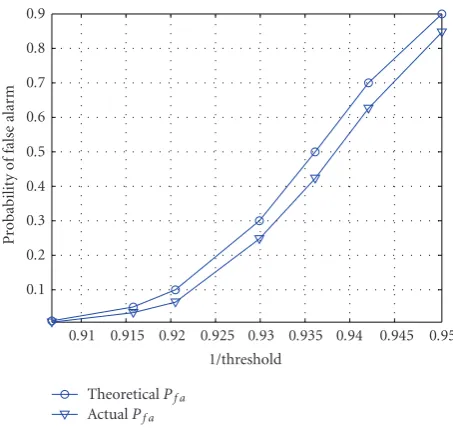
Figure 3shows the expected (theoretical) and actual (by simulation) probability of false alarm values based on the theoretical threshold in (55) for N = 5000, M = 8, and
K =1. It is observed that the differences between these two sets of values are reasonably small, suggesting that the choice of the theoretical threshold is quite accurate.
11. Robust Spectrum Sensing
small deviations from the assumptions. Consequently, the searching for robust detection methods has been of great interest in the field of signal processing and many others [74– 77]. A very useful paradigm to design robust detectors is the maxmin approach, which maximizes the worst case detection performance. Among others, two techniques are very useful for robust cognitive radio spectrum sensing: the robust hypothesis testing [75] and the robust matched filtering [76, 77]. In the following, we will give a brief overview on them, while for other robust detection techniques, the interested readers may refer to the excellent survey paper [78] and references therein.
11.1. Robust Hypothesis Testing. Let the PDF of a received
signal sample be f1 at hypothesisH1 and f0 at hypothesis
H0. If we know these two functions, the LRT-based detection described inSection 2is optimal. However, in practice, due to channel impairment, noise uncertainty, and interference, it is very hard, if possible, to obtain these two functions exactly. One possible situation is when we only know that f1 and f0belong to certain classes. One such class is called the ε-contamination class given by
H0: f0∈F0, F0=
$
(1−0)f0
0 +0g0
% ,
H1: f1∈F1, F1=
$
(1−1)f10+1g1
% ,
(56)
wherefj0(j=0, 1) is the nominal PDF under hypothesisHj,
jin [0, 1] is the maximum degree of contamination, andgj is an arbitrary density function. Assume that we only know
fj0andj(an upper bound for contamination),j=1, 2. The problem is then to design a detection scheme to minimize the worst-case probability of error (e.g., probability of false alarm plus probability of mis-detection), that is, finding a detectorΨ such that
Ψ=arg min
Ψ (f0,fmax1)∈F0×F1
Pf a
f0,f1,Ψ
+ 1−Pd
f0,f1,Ψ
.
(57)
Hubber [75] proved that the optimal test statistic is a “censored” version of the LRT given by
Ψ=TCLRT(x)=
N−1
n=0
r(x(n)), (58)
where
r(t)= ⎧ ⎪ ⎪ ⎪ ⎪ ⎪ ⎪ ⎪ ⎪ ⎪ ⎪ ⎪ ⎪ ⎨ ⎪ ⎪ ⎪ ⎪ ⎪ ⎪ ⎪ ⎪ ⎪ ⎪ ⎪ ⎪ ⎩
c1, c1≤ f 0
1(t)
f0
0(t)
,
f0
1(t)
f0
0(t)
, c0< f 0
1(t)
f0
0(t)
,< c1
c0, f 0
1(t)
f0
0(t)
≤c0,
(59)
andc0,c1are nonnegative numbers related to0,1, f00, and f10[75,78]. Note that if choosingc0 = 0 andc1 =+∞, the test is the conventional LRT with respect to nominal PDFs,
f0
0 andf10.
After this seminal work, there have been quite a few researches in this area [78]. For example, similar minmax solutions are found for some other uncertainty models [78].
11.2. Robust Matched Filtering. We turn the model (4) into a
vector form as
H0:x=η,
H1:x=s+η,
(60)
wheresis the signal vector andηis the noise vector. Suppose that s is known. In general, a matched-filtering detection is TMF = gTx. Let the covariance matrix of the noise be Rη =E(ηηT). IfRη =ση2I, it is known that choosingg=s is optimal. In general, it is easy to verify that the optimalgto maximize the SNR is
g=R−1
η s. (61)
In practice, the signal vectorsmay not be known exactly. For example,smay be only known to be arounds0 with some errors modeled by
s−s0≤Δ, (62)
whereΔis an upper bound on the Euclidean-norm of the error. In this case, we are interested in finding a proper value forgsuch that the worst-case SNR is maximized, that is,
g=arg max
g s:||s−smin0||≤Δ
SNRs,g. (63)
It was proved in [76,77] that the optimal solution for the above maxmin problem is
g=Rη+δI
−1
s0, (64)
whereδis a nonnegative number such thatδ2g2=Δ. It is noted that there are also researches on the robust matched filtering detection when the signal has other types of uncertainty [78]. Moreover, if the noise has uncertainties, that is,Rηis not known exactly, or both noise and signal have uncertainties, the optimal robust matched-filtering detector was also found for some specific uncertainty models in [78].
12. Practical Considerations and
Future Developments
Although there have been quite a few methods proposed for spectrum sensing, their realization and performance in practical cognitive radio applications need to be tested [50– 52]. To build a practical sensing device, many factors should be considered. Some of them are discussed as follows.
(1) Narrowband noise. One or more narrowband filters
noise samples are usually correlated. This will cause many sensing methods unworkable, because they usually assume that the noise samples are i.i.d. For some methods, a noise prewhitening process can be used to make the noise samples i.i.d. prior to the signal detection. For example, this method has been deployed in [22] to enable the eigenvalue-based detection methods. The similar method can be used for covariance-based detection methods, for example, the CAV.
(2)Spurious signal and interference. The received signal
may contain not only the desired signal and white noise but also some spurious signal and interference. The spurious signal may be generated by Analog-to-Digital Convert-ers (ADC) due to its nonlinearity [79] or other inten-tional/unintentional transmitters. If the sensing antenna is near some electronic devices, the spurious signal generated by the devices can be strong in the received signal. For some sensing methods, such unwanted signals will be detected as signals rather than noise. This will increase the probability of false alarm. There are methods to mitigate the spurious signal at the device level [79]. Alternatively, signal processing techniques can be used to eliminate the impact of spurious signal/interference [53]. It is very difficult, if possible, to estimate the interference waveform or distribution because of its variation with time and location. Depending on situations, the interference power could be lower or higher than the noise power. If the interference power is much higher than the noise power, it is possible to estimate the interference first and subtract it from the received signal. However, since we usually intend to detect signal at very low SNR, the error of the interference estimation could be large enough (say, larger than the primary signal) such that the detection with the residue signal after the interference subtraction is still unreliable. If the interference power is low, it is hard to estimate it anyway. Hence, in general we cannot rely on the interference estimation and subtraction, especially for very low-power signal detection.
(3)Fixed point realization. Many hardware realizations
use fixed point rather than floating point computation. This will limit the accuracy of detection methods due to the signal truncation when it is saturated. A detection method should be robust to such unpredictable errors.
(4) Wideband sensing. A cognitive radio device may
need to monitor a very large contiguous or noncontiguous frequency range to find the best available band(s) for transmission. The aggregate bandwidth could be as large as several GHz. Such wideband sensing requires ultra-wide band RF frontend and very fast signal processing devices. To sense a very large frequency range, typically a corresponding large sampling rate is required, which is very challenging for practical implementation. Fortunately, if a large part of the frequency range is vacant, that is, the signal is frequency-domain sparse, we can use the recently developed compressed sampling (also called compressed sensing) to reduce the sampling rate by a large margin [80–82]. Although there have been studies in wideband sensing algorithms [26,83–87], more researches are needed especially when the center frequencies and bandwidths of the primary signals are unknown within the frequency range of interest.
(5)Complexity. This is of course one of the major factors
affecting the implementation of a sensing method. Simple but effective methods are always preferable.
To detect a desired signal at very low SNR and in a harsh environment is by no means a simple task. In this paper, major attention is paid to the statistical detection methods. The major advantage of such methods is their little depen-dency on signal/channel knowledge as well as relative ease for realization. However, their disadvantage is also obvious: they are in general vulnerable to undesired interferences. How we can effectively combine the statistical detection with known signal features is not yet well understood. This might be a promising research direction. Furthermore, most exiting spectrum sensing methods are passive in the sense that they have neglected the interactions between the primary and secondary networks via their mutual interferences. If the reaction of the primary user (e.g., power control) upon receiving the secondary interference is exploited, some active spectrum sensing methods can be designed, which could significantly outperform the conventional passive sensing methods [88,89]. At last, detecting the presence of signal is only the basic task of sensing. For a radio with high level of cognition, further information such as signal waveform and modulation schemes may be exploited. Therefore, signal identification turns to be an advanced task of sensing. If we could find an effective method for this advanced task, it in turn can help the basic sensing task.
13. Conclusion
In this paper, various spectrum sensing techniques have been reviewed. Special attention has been paid to blind sensing methods that do not need information of the source signals and the propagation channels. It has been shown that space-time joint signal processing not only improves the sensing performance but also solves the noise uncertainty problem to some extent. Theoretical analysis on test statistic distribution and threshold setting has also been investigated.
References
[1] FCC, “Spectrum policy task force report,” inProceedings of the Federal Communications Commission (FCC ’02), Washington, DC, USA, November 2002.
[2] M. H. Islam, C. L. Koh, S. W. Oh, et al., “Spectrum survey in Singapore: occupancy measurements and analysis,” in
Proceedings of the 3rd International Conference on Cogni-tive Radio Oriented Wireless Networks and Communications (CROWNCOM ’08), Singapor, May 2008.
[3] J. Mitola and G. Q. Maguire, “Cognitive radio: making soft-ware radios more personal,”IEEE Personal Communications, vol. 6, no. 4, pp. 13–18, 1999.
[4] S. Haykin, “Cognitive radio: brain-empowered wireless com-munications,”IEEE Transactions on Communications, vol. 23, no. 2, pp. 201–220, 2005.
[5] N. Devroye, P. Mitran, and V. Tarokh, “Achieveable rates in cognitive radio channels,”IEEE Transactions on Information Theory, vol. 52, no. 5, pp. 1813–1827, 2006.
[7] C. Stevenson, G. Chouinard, Z. D. Lei, W. D. Hu, S. Shellhammer, and W. Caldwell, “IEEE 802.22: the first cog-nitive radio wireless regional area network standard,” IEEE Communications Magazine, vol. 47, no. 1, pp. 130–138, 2009. [8] Wireless Innovation Alliance, 2008,
http://www.wirelessin-novationalliance.com/.
[9] A. Sonnenschein and P. M. Fishman, “Radiometric detection of spreadspectrum signals in noise of uncertainty power,”IEEE Transactions on Aerospace and Electronic Systems, vol. 28, no. 3, pp. 654–660, 1992.
[10] A. Sahai and D. Cabric, “Spectrum sensing: fundamental limits and practical challenges,” inIEEE International Sympo-sium on New Frontiers in Dynamic Spectrum Access Networks (DySPAN ’05), Baltimore, Md, USA, November 2005. [11] R. Tandra and A. Sahai, “Fundamental limits on detection
in low SNR under noise uncertainty,” inProceedings of the International Conference on Wireless Networks, Communica-tions and Mobile Computing (WirelessCom ’05), vol. 1, pp. 464– 469, Maui, Hawaii, USA, June 2005.
[12] R. Tandra and A. Sahai, “SNR walls for signal detection,”IEEE Journal on Selected Topics in Signal Processing, vol. 2, no. 1, pp. 4–17, 2008.
[13] S. M. Kay, Fundamentals of Statistical Signal Processing: Detection Theory, vol. 2, Prentice Hall, Upper Saddle River, NJ, USA, 1998.
[14] H. Urkowitz, “Energy detection of unkown deterministic signals,”Proceedings of the IEEE, vol. 55, no. 4, pp. 523–531, 1967.
[15] H. S. Chen, W. Gao, and D. G. Daut, “Signature based spectrum sensing algorithms for IEEE 802.22 WRAN,” in
Proceedings of the IEEE International Conference on Commu-nications (ICC ’07), pp. 6487–6492, Glasgow, Scotland, June 2007.
[16] W. A. Gardner, “Exploitation of spectral redundancy in cyclostationary signals,”IEEE Signal Processing Magazine, vol. 8, no. 2, pp. 14–36, 1991.
[17] W. A. Gardner, “Spectral correlation of modulated signals— part I: analog modulation,”IEEE Transactions on Communica-tions, vol. 35, no. 6, pp. 584–595, 1987.
[18] W. A. Gardner, W. A. Brown III, and C.-K. Chen, “Spectral correlation of modulated signals—part II: digital modula-tion,”IEEE Transactions on Communications, vol. 35, no. 6, pp. 595–601, 1987.
[19] N. Han, S. H. Shon, J. O. Joo, and J. M. Kim, “Spectral correlation based signal detection method for spectrum sensing in IEEE 802.22 WRAN systems,” in Proceedings of the 8th International Conference on Advanced Communication Technology, Phoenix Park, South Korea, Febraury 2006. [20] Y. H. Zeng and Y.-C. Liang, “Eigenvalue based sensing
algorithms,” IEEE 802.22-06/0118r0, July 2006.
[21] Y. H. Zeng and Y.-C. Liang, “Maximum-minimum eigenvalue detection for cognitive radio,” in Proceedings of the 18th International Symposium on Personal, Indoor and Mobile Radio Communications (PIMRC ’07), Athens, Greece, September 2007.
[22] Y. H. Zeng and Y.-C. Liang, “Eigenvalue-based spectrum sensing algorithms for cognitive radio,”IEEE Transactions on Communications, vol. 57, no. 6, pp. 1784–1793, 2009. [23] P. Bianchi, J. N. G. Alfano, and M. Debbah, “Asymptotics of
eigenbased collaborative sensing,” inProceedings of the IEEE
Information Theory Workshop (ITW ’09), Taormina, Sicily, Italy, October 2009.
[24] M. Maida, J. Najim, P. Bianchi, and M. Debbah, “Performance analysis of some eigen-based hypothesis tests for collaborative sensing,” inProceedings of the IEEE Workshop on Statistical Signal Processing, Cardiff, Wales, UK, September 2009. [25] F. Penna, R. Garello, and M. A. Spirito, “Cooperative spectrum
sensing based on the limiting eigenvalue ratio distribution in wishart matrices,”IEEE Communications Letters, vol. 13, no. 7, pp. 507–509, 2009.
[26] Z. Tian and G. B. Giannakis, “A wavelet approach to wideband spectrum sensing for cognitive radios,” inProceedings of the 1st International Conference on Cognitive Radio Oriented Wireless Networks and Communications (CROWNCOM ’07), Mykonos, Greece, June 2007.
[27] Y. H. Zeng and Y.-C. Liang, “Covariance based signal detections for cognitive radio,” in Proceedings of the 2nd IEEE International Symposium on New Frontiers in Dynamic Spectrum Access Networks (DySPAN ’07), pp. 202–207, Dublin, Ireland, April 2007.
[28] Y. H. Zeng and Y.-C. Liang, “Spectrum-sensing algorithms for cognitive radio based on statistical covariances,” IEEE Transactions on Vehicular Technology, vol. 58, no. 4, pp. 1804– 1815, 2009.
[29] Y. H. Zeng, Y.-C. Liang, and R. Zhang, “Blindly combined energy detection for spectrum sensing in cognitive radio,”
IEEE Signal Processing Letters, vol. 15, pp. 649–652, 2008. [30] S. Pasupathy and A. N. Venetsanopoulos, “Optimum active
array processing structure and space-time factorability,”IEEE Transactions on Aerospace and Electronic Systems, vol. 10, no. 6, pp. 770–778, 1974.
[31] A. Dogandzic and A. Nehorai, “Cramer-rao bounds for estimating range, velocity, and direction with an active array,”
IEEE Transactions on Signal Processing, vol. 49, no. 6, pp. 1122– 1137, 2001.
[32] E. Fishler, A. Haimovich, R. Blum, D. Chizhik, L. Cimini, and R. Valenzuela, “MIMO radar: an idea whose time has come,” inProceedings of the IEEE National Radar Conference, pp. 71– 78, Philadelphia, Pa, USA, April 2004.
[33] A. Sheikhi and A. Zamani, “Coherent detection for MIMO radars,” inProceedings of the IEEE National Radar Conference, pp. 302–307, April 2007.
[34] P. K. Varshney, Distributed Detection and Data Fusion, Springer, New York, NY, USA, 1996.
[35] J. Unnikrishnan and V. V. Veeravalli, “Cooperative sensing for primary detection in cognitive radio,”IEEE Journal on Selected Topics in Signal Processing, vol. 2, no. 1, pp. 18–27, 2008. [36] G. Ganesan and Y. Li, “Cooperative spectrum sensing in
cognitive radio—part I: two user networks,”IEEE Transactions on Wireless Communications, vol. 6, pp. 2204–2213, 2007. [37] G. Ganesan and Y. Li, “Cooperative spectrum sensing in
cog-nitive radio—part II: multiuser networks,”IEEE Transactions on Wireless Communications, vol. 6, pp. 2214–2222, 2007. [38] Z. Quan, S. Cui, and A. H. Sayed, “Optimal linear cooperation
for spectrum sensing in cognitive radio networks,” IEEE Journal on Selected Topics in Signal Processing, vol. 2, no. 1, pp. 28–40, 2007.