R E S E A R C H
Open Access
An active noise control algorithm with gain and
power constraints on the adaptive filter
Walter J Kozacky and Tokunbo Ogunfunmi
*Abstract
This article develops a new adaptive filter algorithm intended for use in active noise control systems where it is required to place gain or power constraints on the filter output to prevent overdriving the transducer, or to maintain a specified system power budget. When the frequency-domain version of the least-mean-square algorithm is used for the adaptive filter, this limiting can be done directly in the frequency domain, allowing the adaptive filter response to be reduced in frequency regions of constraint violation, with minimal effect at other frequencies. We present the development of a new adaptive filter algorithm that uses a penalty function formulation to place multiple constraints on the filter directly in the frequency domain. The new algorithm performs better than existing ones in terms of improved convergence rate and frequency-selective limiting.
Keywords:Adaptive filtering, Adaptive signal processing, Discrete fourier transforms, FXLMS, Optimization
1. Introduction
Active noise control (ANC) systems can be used to re-move interference by generating an anti-noise output that can be used in the system to destructively cancel the interference [1]. In some applications, it is required to limit the maximum output level to prevent overdriv-ing the transducer, or to maintain a specified system power budget. In a frequency-domain implementation of the least-mean-square (LMS) algorithm, the limiting constraints can be placed directly in the frequency do-main, allowing the adaptive filter response to be reduced in the frequency regions of constraint violation, with minimal effect at other frequencies [2]. Constraints can be placed on either the filter gain, or filter output power, as appropriate for the application.
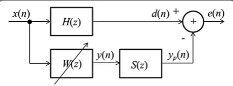
A general block diagram of an ANC system is illustrated in Figure 1, with H(z) representing the pri-mary path or plant (e.g., an acoustic duct), W(z) representing the adaptive filter, andS(z) representing the secondary path (which may include the D/A converter, power output amplifier, and the transducer). The adap-tive filter W(z) typically uses the filtered-X LMS algo-rithm, where the input to the LMS algorithm is first filtered by an estimate of the secondary path [3]. The adaptive filter will need to simultaneously identify H(z)
and equalize S(z), with the additional constraint of limiting the maximum level delivered toS(z).
Applications of gaconstrained adaptive systems in-clude systems that use a microphone for feedback, and due to the acoustic path to the microphone notches or peaks occur in the microphone frequency response (which may not be present in other locations). Adding gain constraints to the adaptive filter prevents distortion at those frequencies by limiting the peak magnitude of the filter coefficients [2]. Applications of power-constrained adaptive systems include requirements to limit the maximum power delivered to S(z) to a predetermined constraint value to prevent overdriving the transducer, prevent output amplifier saturation, or prevent other nonlinear behavior [4]. The primary differ-ence between these implementations is that the gain-constrained algorithm does not take the input power into account when determining the constraint violation.
Previous implementations of gain and output power limiting include output rescaling, the leaky LMS, and a class of algorithms termed constrained steepest descent (CSD) previously presented in [2]. We develop a new class of gain-constrained and power-constrained algorithms termed constrained minimal disturbance (CMD). The new CMD algorithms provide faster convergence compared to previous algorithms, and the ability to handle multiple constraints.
* Correspondence:[email protected] Santa Clara University, Santa Clara, CA, USA
This article is organized as follows. Section 2 presents a review of prior work. Section 3 presents the CMD algorithm development. Section 4 presents a convergence analysis. Section 5 presents simulations with comparisons to other algorithms. Section 6 provides some concluding remarks.
2. Review of prior work
For comparison purposes, the following notation is used.
n Adaptive filter size and block size
N Sample number in the time domain
m Block number in the time or frequency domain
W Weight in the frequency domain
X Input in the frequency domain
E Error in the frequency domain
D Plant output in the frequency domain
Y Filter output in the frequency domain
C Gain or power constraint
S Secondary path
Lowercase w, x, e, d, and y are the time-domain representations of their respective frequency-domain counterparts. Vectors will be denoted in boldface, and the subscript k is used to denote an individual compo-nent of a vector. The superscript * is used to denote complex conjugate, and the superscriptTdenotes vector transpose. The parameter μ is used as a convergence step-size coefficient, and the parameter γ is used as a leakage coefficient.
The first two methods of power limiting were described in detail in [5] and are briefly restated here. The first “output clipping” simply limits the output power to a maximum value. This is what would nor-mally happen in a real system (e.g., the output amplifier would saturate). With the filter output y at iteration n
denoted byy(n) and the output constraint byC, the out-put clipping algorithm is given by
if y nð þ1Þ>C
y nð þ1Þ ¼y nð þ1Þ C
y nð þ1Þ
j j:
ð1Þ
A potential problem in using output clipping for adap-tive filtering applications is that the weight updates for
w(n) continue to occur while the filter output remains clipped, causing potential stability problems since the fil-ter weight update is decoupled from the filfil-ter output. To prevent this, the ”output re-scaling” algorithm can be used, which is given by
if y nð þ1Þ>C
y nð þ1Þ ¼y nð þ1Þ C
y nð þ1Þ
j j
wðnþ1Þ ¼wðnþ1Þ C
y nð þ1Þ
j j:
ð2Þ
Here, in addition to the output being clipped, the adap-tive filter weights are also rescaled; filter adaptation continues from the appropriate weight value corresponding to the actual output.
The next algorithm to be considered for gain or power limiting is the leaky LMS [6], which is given by
wðnþ1Þ ¼ð1μγÞwð Þ þn μe nð Þxð Þn: ð3Þ
The leaky LMS reduces the filter gain each iteration, with the leakage coefficient γcontrolling the rate of re-duction. The coefficient γ is determined experimentally according to the application, but gain reduction occurs at all frequencies, resulting in a larger steady-state con-vergence error. When the leakage is zero, this algorithm reduces to the standard LMS [7].
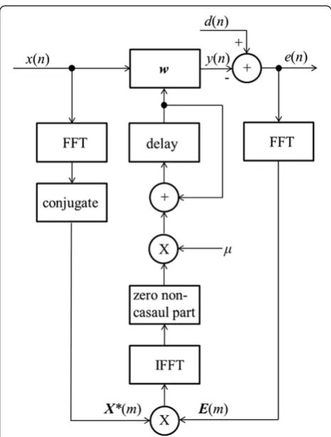
The algorithms described thus far are processed dir-ectly in the time domain. However, with large filter lengths the required convolutions become computation-ally expensive, and alternative methods can be more effi-cient. If the processing is done in block form and a fast Fourier transform (FFT) used, the required convolutions become multiplications. This also allows additional constraints to be added to limit the filter response dir-ectly in the frequency domain. For example, in [8], an ANC system using a loudspeaker with poor low-frequency response was stabilized in the FFT domain by zeroing out the low-frequency components, preventing adaptation at those frequencies. However, using block processing will result in a one block delay, which may be undesirable in some real-time applications. A delayless structure [9], with filtering in the time-domain and sig-nal processing in the frequency-domain, can be used to mitigate this delay. A block diagram of the delayless frequency-domain LMS (FDLMS) is shown in Figure 2. In delayless ANC applications with a secondary path
by an estimate of the secondary path. The adaptive filter weight, input, and error vectors are defined as
wð Þ ¼m ½w0ð Þnw1ð Þn . . .wN1ð Þn T
xð Þ ¼m ½x nð Þx nð 1Þ. . .x nð Nþ1ÞT
eð Þ ¼m ½e nð Þe nð 1Þ. . .e nð Nþ1ÞT ð4Þ
A block size of Nis used for both the filter and each new set of data to maximize computational efficiency, withmrepresenting the block iteration. To avoid circu-lar convolution effects, each FFT uses blocks of size 2N
[10]. The frequency-domain input and error vectors (size 2N) are defined as
Xð Þ ¼m FFTn½xTðnNÞ xTð ÞnTo Eð Þ ¼m FFTn½0 eTð ÞnTo;
ð5Þ
where0is theN-point zero vector.
The delayless FDLMS weight update equation at iter-ation m without a gain or power constraint is given by [9]
wðmþ1Þ ¼wð Þ þm μIFFTfXð Þm Eð Þm gþ; ð6Þ
where the + subscript denotes the causal part of the IFFT (corresponding to the gradient constraintin [10]), andμ is the convergence coefficient. Adding a leakage factor to (6) results in a frequency-domain version of the leaky LMS which can be used to limit the adaptive filter out-put [2], and is given by
wðmþ1Þ ¼γwð Þ þm μIFFTfXð Þm Eð Þm gþ ð7Þ
whereγis the leakage factor.
The next two weight update equations were developed in [2], which processes the constraints in the frequency domain using an algorithm based on the method of steepest descent. The delayless form of the gain-constrained version is given by
wðmþ1Þ ¼wð Þm
þμIFFT Xð ÞmEð Þ m 4αNWð Þm2CzWð Þm
n o
þ ð8Þ
where thezsubscript sets the result in the brackets to 0 if the value in the brackets is less than 0 (the constraint is satisfied), or to the value of the difference (the con-straint is violated). The concon-straint is individually applied to each frequency bin. Here,αcontrols the“tightness”of the penalty: a larger α places a stiffer penalty on con-straint violation at the expense of a larger steady-state convergence error.
The delayless form of the power-constrained algorithm is given by
wðmþ1Þ ¼wð Þm
þμIFFTXð ÞmEð Þ m 4α½P mð Þ CZXð Þm2Wð Þmþ:
ð9Þ
The output power P(m) is determined by the squared Euclidean norm of the filter output, which is required to be limited to a constraint valueC, or equivalently
P mð Þ ¼yð Þm 2<C: ð10Þ
Note that in (10) there is only one constraint. When used for comparison purposes, we will denote (8) and (9) as constrained steepest descent (CSD) algorithms.
3. New algorithm development
The new CMD algorithm will be developed using the
principle of minimal disturbance, which states that the Figure 2Block diagram of the delayless ANC system with
weight vector should be changed in a minimal manner from one iteration to the next [11]. A constraint is added for filter convergence, and a constraint is also added for either the filter gain (coefficient’s magnitude in each fre-quency bin), or the filter output power, depending on which we intend to limit. The method of Lagrange multipliers [11,12] is then used to solve this constrained optimization problem [13].
3.1. Gain-constrained algorithm
At each block update m, the new algorithm will minimize the squared Euclidean norm of the frequency-domain weight change in each individual frequency bin
k, where the weight change is given by
δWkðmþ1Þ ¼Wkðmþ1Þ Wkð Þm; ð11Þ
subject to the condition ofa posteriorifilter convergence in the frequency domain
Dkð Þ ¼m Skð Þm Wkðmþ1ÞXkð Þm: ð12Þ In gain-constrained applications, the algorithm will add-itionally add a penalty based on the amount of magnitude violation above a maximum constraint value, requiring
Wkðmþ1Þ j j≤ ffiffiffiffiffiffiCk
p
ð13Þ
or equivalently
Wkðmþ1Þ2≤Ck: ð14Þ
The three requirements given by (11), (12), and (14) are combined into a single cost function, written as
J mð þ1Þ ¼δWkðmþ1Þ2
þRefλ½Dkð Þ m Skð ÞmWkðmþ1ÞXkð Þm g
þαmax;k Wkðmþ1Þ2Ck
2
h i
z
ð15Þ
where the Lagrange multiplier λ controls the conver-gence requirement of (12), and the Lagrange multiplier αmax,k with subscriptkcontrols the individual frequency
bin magnitude constraint; parameter αmax,k controls the
“tightness” of the penalty term, with a larger value pla-cing more emphasis on meeting the constraint at the ex-pense of increasing the convergence error [2]. The cost function (15) is differentiated with respect to each of the three variables and set to 0. For each frequency bink
∂J mð þ1Þ ∂Wkðmþ1Þ
¼2½Wkðmþ1Þ Wkð ÞmλSkð ÞmXkð Þm
þ2αkWkðmþ1Þ Wkðmþ1Þ2Ck
z¼0
ð16Þ
∂J mð þ1Þ
∂λ ¼Dkð Þ m Skð ÞmWkðmþ1ÞXkð Þ ¼m 0 ð17Þ
∂J mð þ1Þ
∂αmax;k ¼ Wkðmþ1Þ
2
Ck
2
h i
z¼0: ð18Þ Rearranging (16) gives
1þ2αmax;k Wkðmþ1Þ2Ck
z
Wkðmþ1Þ
¼Wkð Þ þm 1
2λ
Skð ÞmXkð Þm:
ð19Þ
We now propose the following interpretation of the gain-constraint term. In steady state (after convergence), we would expect the successive weight values to be approxi-mately the same for a small convergence coefficient step size. Therefore, as long as the constraint of (14) was satisfied in the previous iteration, the penalty is set to 0. However, if the magnitude of the filter weight exceeds the constraint value, then the penalty is scaled in proportion to the con-straint violation (similar to the method in [14], which initiates the penalty at 90% of the constraint). We define
αk¼2αmax;k Wkð Þm2Ck
z ð20Þ
where thezsubscript term will forceαkto zero if the
con-straint of (14) is satisfied.
Substituting (20) into (19) at frequency bin k, conju-gating both sides, and rearranging into a recursion results in
Wkðmþ1Þ ¼ 1 1þαk
½ Wkð Þ þm
1 2λS
kð ÞmX
kð Þm
:
ð21Þ
Substituting (21) into (12) gives
Dkð Þ m Sk
1 1þαk
½ Wkð Þ þm
1 2λS
kð ÞmX
kð Þm
Xkð Þ ¼m 0:
ð22Þ
Rearranging (22) yields
Dkð Þ m Skð Þm Wkð ÞmXkð Þm
½
þαkDkð Þ m 1
2λkSkð Þmk 2 X
kð Þm
k k2¼0:
ð23Þ
The first term in brackets is the error at frequency bin
k,Ek(m). Solving forλresults in
λ¼2½Ekð Þ þm αkDkð Þm Skð Þm 2Xkð Þm 2
Rearranging (21) into a recursion, using (24), and introducing a convergence step size parameterμto con-trol the rate of adaptation yields
Wkðmþ1Þ
¼ 1
1þαk
Wkð Þ þm μ
Ekð Þ þm αkDkð Þm
½
Skð Þm2Xkð Þm
Skð ÞmXkð Þm
" #
:
ð25Þ
Noting thatDk(m) in (25) can be written asDk(m) =Ek
(m) +SkWk(m)Xk(m) results in
Wkðmþ1Þ ¼
1þμαk 1þαk
Wkð Þm
þ μ
Skð Þm2Xkð Þm 2
Skð ÞmXkð Þm Ekð Þm : ð26Þ
For smallμ, (26) can be approximated as
Wkðmþ1Þ ¼ 1 1þαk
Wkð Þm
þ μ
Skð Þm2Xkð Þm2
Skð Þm Xkð ÞmEkð Þm : ð27Þ
Using the definitions
γk ¼ αk μð1þαkÞ
ð28Þ
and
μk ¼
μ
Skð Þm 2Xkð Þm 2
ð29Þ
the weight update given by (27) can be written for each frequency bin as
Wkðmþ1Þ ¼ 1μγk
Wkð Þm
þμkSkð ÞmXkð Þm Ekð Þm :
ð30Þ
Taking the IFFT of both sides and casting into a delayless structure results in the new CMD algorithm given by
wðmþ1Þ ¼wð Þm
þμIFFT Sð Þm X
ð ÞmEð Þm
Sð Þm 2Xð Þm2 Γð Þm Wð Þm
( )
þ ð31Þ
where
Γð Þ ¼m diagγ0ð Þm ;γ1ð Þm ;. . .;γ2N1ð Þm ð32Þ is a diagonal matrix of variable leakage factors as determined by (28).
The ║X(m)║2 term provides an estimate of the input powerPx,k(m) in frequency bink,
Px;kð Þ ¼m E Xkð Þm 2
ð33Þ
which can be determined recursively by [15]
Px;kð Þ ¼m βPx;kðm1Þ
þð1βÞ Xkð Þm Xkð Þm
ð34Þ
where β is a smoothing constant slightly less than 1. (Note: In equations such as (31) which use an estimated power value in the denominator, low power in a particu-lar frequency bin may result in division by a very small number, potentially causing numerical instability. To guard against this, a small positive regularization param-eter is added to the denominator to ensure numerical stability [11]).
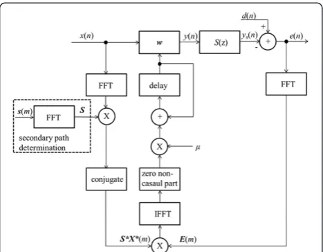
The following observations can be made of the CMD algorithm given by (31), which is shown in Figure 3:
1. If the constraint of (14) is violated, the CMD algorithm will reduce the magnitude of the adaptive filter frequency response in proportion to the level of constraint violation.
2. The CMD algorithm normalizes the weight update in a manner similar to the normalized-LMS with leakage. The amount of leakage is dependent on the level of constraint violation.
3. The CMD algorithm scales the weight update by the inverse of secondary path frequency response, resulting in a faster convergence in regions corresponding to valleys (low magnitude response) in the secondary path.
3.2. Power-constrained algorithm
In applications where the filter output power is to be limited, the gain coefficient constraint is replaced by an output power constraint. If total control effort is to be limited [2,6], a single output power constraint can be expressed as
Pyðmþ1Þ≤C ð35Þ
where
Pyðmþ1Þ ¼ 1
N
X
N1
k¼0
The new power constrained cost function then becomes
J mð þ1Þ ¼δWkðmþ1Þ2
þRe
λhD
kð Þ m Skð ÞmWkðmþ1ÞXkð Þm
i
þαmax;k Pyðmþ1Þ C
2
h i
z: ð37Þ Following the development of the gain-constrained al-gorithm, this cost function is differentiated with respect to each of the three variables and set to 0. The resulting equations are
∂J mð þ1Þ ∂Wkðmþ1Þ
¼2½W mð þ1Þ Wkð ÞmλSkð ÞmXkð Þm
þ2αkWðmþ1ÞXkð Þm2Pyðmþ1Þ C
z¼0
ð38Þ
∂J mð þ1Þ
∂λ ¼Dkð Þ m Skð ÞmWkðmþ1ÞXkð Þ ¼m 0 ð39Þ
∂J mð þ1Þ ∂αmax;k
¼ Pyðmþ1Þ C
2
h i
z¼0: ð40Þ Rearranging (38) yields
2αmax;kXkð Þm2 Pyðmþ1Þ C
z
Wkðmþ1Þ
þWkðmþ1Þ
¼Wkð Þ þm 1
2λ
Skð Þm Xkð Þm : ð41Þ
Using the same procedure previously described after (19), the term in (20) is replaced by
αk¼2αmax;kXkð Þm 2 Py;kð Þ m Ck
z: ð42Þ
Following a development similar to the gain-constrained case results in the CMD algorithm given by (31) using a new diagonal matrix of leakage factors (32).
Better frequency performance can be achieved by esti-mating the power in each frequency bin, making the al-gorithm more selective in attenuating those frequencies in violation of the constraint. The output power in each frequency bin is determined by
Py;kðmþ1Þ ¼Wkðmþ1Þ2Px;kðmþ1Þ: ð43Þ UsingCkas the power constraint, it is required that
Py;kðmþ1Þ≤Ck: ð44Þ
The resulting cost function is given by
J mð þ1Þ ¼δWkðmþ1Þ2
þRefλ½Dkð Þ m Skð Þm Wkðmþ1ÞXkð Þm g
þαmax;k Py;kðmþ1Þ Ck
2
h i
z:
ð45Þ
Following the development of the gain-constrained al-gorithm, this cost function is differentiated with respect to each of the three variables and set to 0. The resulting equations are
∂J mð þ1Þ ∂Wkðmþ1Þ
¼2½Wkðmþ1Þ Wkð ÞmλSkð ÞmXkð Þm
þ2αkWkðmþ1ÞXkð Þm2Py;kðmþ1Þ Ck
z¼0
ð46Þ ∂J mð þ1Þ
∂λ ¼Dkð Þ m Skð ÞmWkðmþ1ÞXkð Þ ¼m 0 ð47Þ
∂J mð þ1Þ
∂αmax;k ¼ Py;kðmþ1Þ Ck
2
h i
z¼0: ð48Þ
Rearranging (46) yields
2αmax;kXkð Þm2 Py;kðmþ1Þ Ck
z
Wkðmþ1Þ
þWkðmþ1Þ
¼Wkð Þ þm
1 2λ
S
kð ÞmXkð Þm:
ð49Þ Figure 3Block diagram of the CMD adaptive filter with
Using the same procedure previously described after (19), the term in (20) is replaced by
αk ¼2αmax;kXkð Þm 2 Py;kð Þ m Ck
z: ð50Þ
Following a development similar to the gain-constrained case, and using a new diagonal matrix of leakage factors (32) results in the CMD algorithm, repeated below.
wðmþ1Þ ¼wð Þm
þμIFFT S
ð Þm Xð ÞmEð Þm
Sð Þm2Xð Þm 2 Γð Þm Wð Þm
( )
þ ;
ð51Þ
where
Γð Þ ¼m diagγ0ð Þm;γ1ð Þm ;. . .;γ2N1ð Þm: ð52Þ
4. Convergence analysis
We assume that all signals are white, zero-mean, Gaussian wide-sense stationary, and employ the independence as-sumption [7] under a steady-state condition, where the constraint violation is constant and the transform-domain weights are mutually uncorrelated (which occurs as the fil-ter sizeNgrows large [16]). We will also use a normalized input power of unity in (34), which then allows the ana-lysis to apply to both gain-constrained and power-constrained cases. Uncorrelated white measurement noise with a variance ofσn2will be denoted byηk.
4.1. Mean value
The weight update equation (30) can be written as
Wkðmþ1Þ ¼ 1μγk
Wkð Þm
þμk½Dkð Þ m Skð ÞmWkð Þm Xkð Þm Skð Þm X kð Þm
ð53Þ or equivalently
Wkðmþ1Þ ¼ 1μ γkþ1
Wkð Þ þm μWk;opt; ð54Þ
whereWk,optdenotes the optimal Wiener solution [given as Sk–1 (m)Dk (m)]. Taking expectations of both sides,
using the assumptions, and noting that the input power is normalized per (29) results in
E W½ kðmþ1Þ ¼ 1μ γkþ1
E W½ kð Þm þμWk;opt ð55Þ
By induction, this recursion can be written as
E W½ kð Þm ¼ 1μ γkþ1
m
E W½ kð Þ0
þμWk;opt
X
m1
i¼0
1μ γ kþ1
m1i ð56Þ
Convergence requirements onμare given below. When these conditions are satisfied the result is
lim
m→1E W½ kð Þm ¼μWk;optmlim→1
X
m1
i¼0
1μ γ kþ1
m1i;
ð57Þ
which converges in the limit to the steady-state solution
Wk,ss.
Wk;ss¼
Wk;opt
1þγk ð58Þ
4.2. Convergence in the mean
The deviation from the steady-state solution in bin kis defined by a weight error [17] given by
Vkð Þ ¼m Wkð Þ m Wk;ss ð59Þ
allowing the CMD algorithm to be expressed as
Vkðmþ1Þ ¼ 1μγkμkX
kð Þm Xkð Þm
Vkð Þm þμkηkXkð Þ m μγkWk;ss
ð60Þ
Taking expectations of both sides results in
E V½ kðmþ1Þ ¼ 1μ γkþ1
E V½ kð Þm μγkWk;ss ð61Þ
By induction, this recursion can be written as
E V½ kð Þm ¼ 1μ γkþ1
m
E V½ kð Þ0
μγkWk;ss
X
m1
i¼0
1μ γ kþ1
m1i
ð62Þ
For this to converge requires the exponential term to decay
1μ γ kþ1
<1 ð63Þ
resulting in
μ< 2
1þγk ð64Þ
with the upper bound onμoccurring for maximum con-straint violation, given by
μ< 2
4.3. Convergence in the mean square
Both sides of (60) are first post-multiplied by their re-spective conjugate transposes, rearranged, and after tak-ing expectations the result is
E Vkðmþ1ÞVkðmþ1Þ
¼E 1μγkμk 2
Vkð ÞmVkð Þm
h i
þ μ2σ2n Xkð Þm2
þμ2γ2
kWk;ssWk;ss
μγkE 1μγkμk
Vkð ÞmWk;ss
h i
μγkE 1μγkμk
Vkð ÞmWk;ss
ð66Þ
Rearranging and employing the assumptions [18] gives
E Vkðmþ1ÞVkðmþ1Þ
¼ ½ 12μ γ kþ1þμ2 γ2
kþ2γkþ1
E Vkð ÞmVkð Þm
þ μ2σ2n Xkð Þm 2
þμ2γ2
kWk;ssð Þm 2
2μγk 1μ γkþ1
Wk;ssE V½ kð Þm: ð67Þ
As the weight error variance update depends on the mean coefficient error vector,Vk(m), a state-space model
can be defined as
Zkð Þ ¼m E Vkð ÞmV kð Þm
E V½ kð Þm
ð68Þ
and the update defined as the real component of
Zkðmþ1Þ ¼AZkð Þ þm B ð69Þ
with
A¼ A11 A12 0 A22
ð70Þ
and
B¼ B1
B2
ð71Þ
where
A11¼12μ γkþ1
þμ2 γ2
kþ2γkþ1
A12¼ 2μγk 1μ γkþ1
Wk;ss
A22¼1μ γkþ1
B1¼μ2 σ 2 n Xkð Þm2
þγ2
kWk;ssð Þm2
!
B2¼ μγkWk;ss:
ð72Þ
For stability, it is required that the eigenvalues in the state transition matrix A have a magnitude less than 1
0 0.1 0.2 0.3 0.4 0.5 0.6 0.7 0.8 0.9 1 -40
-30 -20 -10 0 10 20
P
o
we
r (d
B
)
Normalized Frequency Ideal unconstrained filter
CMD Algorithm
[19], requiring matrix entryA11in (70) to be bounded to magnitude less than 1, resulting in
12μ γ kþ1þμ2γ2kþ2γkþ1
<1 ð73Þ
or
μ< 2
1þγk ð74Þ
with the upper bound onμoccurring for maximum con-straint violation, given by
μ< 2
1þγk;max ð75Þ
5. Simulations
In the simulations, the experimental data from [3] is used for the plant, modeled by a 512-term all-zero filter centered at N/2. The output rescaling algorithm (2) is 0 0.1 0.2 0.3 0.4 0.5 0.6 0.7 0.8 0.9 1
-40 -30 -20 -10 0 10 20
P
o
we
r (d
B
)
Normalized Frequency Plant
Secondary Path
CMD Algorithm
Figure 5Frequency response of gain-constrained CMD algorithm with secondary path.
0 1000 2000 3000 4000 5000 6000 10-6
10-5 10-4 10-3 10-2 10-1 100
Bl
o
c
k
Av
e
ra
g
e
d
M
SE (
d
B)
Block Number CMD Algorithm
CSD Algorithm Leaky LMS
applied in the frequency-domain to determine the steady-state adaptive filter final coefficients. We demonstrate the improved convergence performance of the CMD algo-rithm as compared to the CSD algoalgo-rithm and the leaky LMS in both gain-constrained and power-constrained applications. The values of constraint terms C, αmaxk,
andCkare held constant in the simulations, but could be
shaped over frequency for specific applications. External uncorrelated Gaussian white noise with a variance of 0.01
is added for the convergence comparisons, and an average of 100 runs is plotted. In the simulations, we are assuming prior knowledge of the secondary path transfer function; methods for on-line and off-line secondary path identifica-tion are presented in, e.g., [20,21].
5.1. Gain-constrained algorithm
Using a unity gain secondary path, a 3-dB coefficient gain constraint is imposed, and Figure 4 shows the plant 0 500 1000 1500 2000 2500 3000
10-6 10-5 10-4 10-3 10-2 10-1 100
Bl
o
c
k
Av
e
ra
g
e
d
M
SE (
d
B)
Block Number Leaky LMS
CSD Algorithm
CMD Algorithm
Figure 7Convergence comparison, gain-constrained condition, AR(1) colored noise input.
0 0.1 0.2 0.3 0.4 0.5 0.6 0.7 0.8 0.9 1 -80
-70 -60 -50 -40 -30 -20 -10 0 10 20
Po
w
e
r (
d
B)
Ideal unconstrained filter
CMD Algorithm CSD Algorithm Leaky LMS
Normalized Frequency
frequency response and the response of the new CMD algo-rithm, illustrating the clipping effect of the algorithm.
Using the experimental data from [3] for the second-ary path, the algorithms should converge to the filter in Figure 5, which shows the CMD algorithm re-sponse, the plant frequency rere-sponse, and the secondary path frequency response. The adaptive filter in this case will need to simultaneously identify H(z) and equalize
S(z), while still maintaining the gain constraints. The
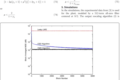
convergence comparison for the three algorithms for the system in Figure 5 for a white noise input is displayed in Figure 6. The CMD algorithm has the fastest convergence performance. The CSD algorithm began converging in a similar manner, but was not able to fully achieve the relatively high 20 dB gain required at the lowest frequen-cies in Figure 5. However, other simulations without deep secondary path nulls showed that the two algorithms con-verge to similar final weight values, with the CMD having 0 50 100 150 200 250 300 350 400 450 500
10-6 10-5 10-4 10-3 10-2 10-1 100
Bl
o
c
k
Av
e
ra
g
e
d
M
SE (
d
B)
Block Number Leaky LMS
CSD Algorithm
CMD Algorithm
Figure 9Convergence comparison, power-constrained condition.
0 0.1 0.2 0.3 0.4 0.5 0.6 0.7 0.8 0.9 1 -40
-30 -20 -10 0 10 20
Po
w
e
r (
d
B)
Normalized Frequency Ideal unconstrained filter
CMD Algorithm
a faster convergence rate. The leaky LMS attenuates all fre-quencies (and not just those in violation of the constraint) and has the poorest convergence performance. (The leaky LMS appears smoother than the other two algorithms, but this is due to the logarithmic scale of the y-axis in the plots.)
Figure 7 compares the convergence of the three algorithms for colored noise input, created by filtering the input with a first order AR(1) low pass filter process with coefficients [1–0.95]. The CSD algorithm requires a significant reduction of μ in (8) to maintain stability, resulting in a slow response. However, the increased energy in the lower frequency regions due to the low pass input process improved the misadjustment for this case. The leaky LMS attenuates all frequencies (and not just those in violation of the constraint) and has the poorest convergence performance and highest excess misadjustment.
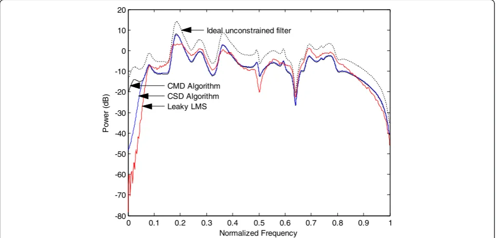
5.2. Power-constrained algorithm
The frequency response and convergence of the three algorithms is compared in Figures 8 and 9, respectively, using a single output power constraint of 25% of the un-constrained value (−6 dB). The CMD algorithm has the fastest convergence performance and maintains a 6-dB power reduction over frequency. The CSD displays simi-lar performance, but again was not able to fully achieve the relatively high 20 dB gain required at the lowest fre-quencies. The leaky LMS has the poorest convergence performance, primarily due to its inability to track the lowest frequencies. Both the CMD and CSD algorithms allow the power constraint to be set explicitly, while the leaky LMS requires a trial and error approach to deter-mine the parameters.
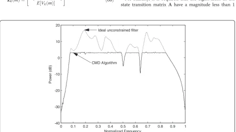
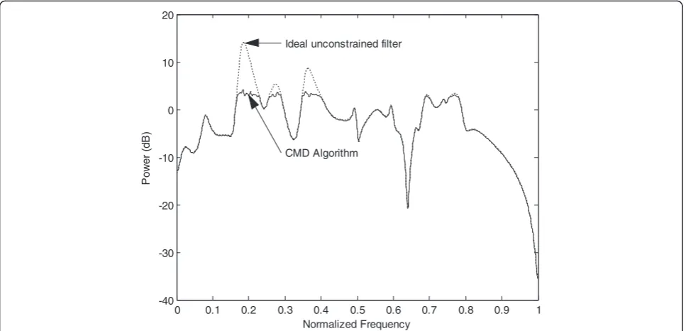
The CMD algorithm frequency response for the indi-vidual bin-constrained case using the constraint of (44) is shown in Figure 10 for a 3-dB power limit with a wideband white noise input. Comparing this to Figure 8 illustrates how the new CMD algorithm reduces the out-put in the frequencies of power-constraint violation, while minimizing the effect at other frequencies.
6. Conclusion
A new algorithm was presented, the CMD LMS, for gain-constrained and power-constrained adaptive filter applications. Analysis results were developed for the stabil-ity bounds in the mean and mean-square sense. The CMD algorithm was compared to the algorithm developed in [2] and the leaky LMS for filtered-X ANC applications. The new CMD algorithm provides faster convergence and improved frequency response performance, especially in colored noise environments. Additionally, the new CMD algorithm has the ability to handle multiple constraints in both gain-constrained and power-constrained applications.
Competing interests
The authors declare that they have no competing interests.
Authors’contribution
WJK and TO derived the equations, carried out and reviewed the simulations, and drafted the manuscript. Both authors read and approved the final manuscript.
Received: 2 May 2012 Accepted: 21 January 2013 Published: 11 February 2013
References
1. PA Nelson, SJ Elliott,Active Control of Sound(Academic Press, London, 1992) 2. B Rafaely, S Elliot, A computationally efficient frequency-domain LMS
algorithm with constraints on the adaptive filter. IEEE Trans. Signal Process. 48(6), 1649–1655 (2000)
3. SM Kuo, DR Morgan,Active Noise Control Systems: Algorithms and DSP Implementations(Wiley, New York, 1996)
4. F Taringoo, J Poshtan, MH Kahaei, Analysis of effort constraint algorithm in active noise control systems. EURASIP J. Appl. Signal Process.2006, 1–9 (2006) 5. X Qiu, CH Hansen, A study of time-domain FXLMS algorithms with control
output constraint. J. Acoust. Soc. Am.1097(6), 2815–2823 (2001) 6. P Darlington, Performance surfaces of minimum effort estimators and
controllers. IEEE Trans. Signal Process.43(2), 536–539 (1995) 7. B Widrow,SD Stearns: Adaptive Signal Processing(Prentice-Hall, Upper
Saddle River, NJ, 1985)
8. MP Nowak, BD Van Veen, A constrained transform-domain adaptive IIR filter structure for active noise control. IEEE Trans. Speech Audio Process. 5(5), 334–347 (1997)
9. DR Morgan, JC Thi, A delayless subband adaptive filter architecture. IEEE Trans. Signal Process.43(8), 1819–1830 (1995)
10. JJ Shynk, Frequency-domain and multirate adaptive filtering. IEEE Signal Process. Mag.9, 337–339 (1993)
11. S Haykin,Adaptive Filter Theory(Prentice-Hall, Upper Saddle River, NJ, 2002) 12. R Fletcher,Practical Methods of Optimization(Wiley, New York, 1987) 13. WJ Kozacky, T Ogunfunmi, Convergence analysis of a frequency-domain
adaptive filter with constraints on the output weights, inProceedings of the Asilomar Conference on Signals, Systems, and Computers(Pacific Grove, USA, 2009), pp. 1350–1355
14. SJ Elliott, KH Beck, Effort constraints in adaptive feedforward control. IEEE Signal Process. Lett.3(1), 7–9 (1996)
15. PCW Sommen, PJ Van Gerwen, HJ Kotmans, JEM Janssen, Convergence analysis of a frequency-domain adaptive filter with exponential power averaging and generalized window function. IEEE Trans. Circuits Syst. 34(7), 788–798 (1987)
16. B Farhang-Boroujeny, KS Chan, Analysis of the frequency-domain block LMS algorithm. IEEE Trans. Signal Process.48(8), 2332–2342 (2000)
17. K Mayyas, T Aboulnast, Leaky LMS algorithm: MSE analysis for Gaussian data. IEEE Trans. Signal Process.45(4), 927–934 (1997)
18. SC Douglas, Performance comparison of two implementations of the leaky LMS adaptive filter. IEEE Trans. Signal Process.45(8), 2125–2129 (1997) 19. K Mayyas, T Aboulnasr, Leaky LMS: a detailed analysis, inProceedings of the
IEEE International Symposium on Circuits and Systems (ISCAS). Seattle, USA2, 1255–1258 (1995)
20. SM Kuo, D Vijayan, A secondary path modeling technique for active noise control systems. IEEE Trans. Speech Audio Process.5(4), 374–377 (1997) 21. MT Akhtar, M Abe, M Kawamata, On active noise control systems with
online acoustic feedback path modeling. IEEE Trans. Audio Speech Lang. Process.15(2), 593–600 (2007)
doi:10.1186/1687-6180-2013-17
Cite this article as:Kozacky and Ogunfunmi:An active noise control algorithm with gain and power constraints on the adaptive filter.