Volume 2010, Article ID 751069,7pages doi:10.1155/2010/751069
Research Article
Application of Linear Prediction Technique to Passive Synthetic
Aperture Processing
Yunshan Hou, Jianguo Huang, Min Jiang, and Yong Jin
College of Marine Engineering, Northwestern Polytechnical University, 710072 Xi’an, China
Correspondence should be addressed to Yunshan Hou,[email protected]
Received 10 October 2009; Accepted 15 February 2010
Academic Editor: M. Greco
Copyright © 2010 Yunshan Hou et al. This is an open access article distributed under the Creative Commons Attribution License, which permits unrestricted use, distribution, and reproduction in any medium, provided the original work is properly cited.
A method for the synthesis of an aperture with improved angular resolution and array gain is described. The proposed method explores the merit of linear prediction technique to improve the performance of conventional ETAM (extended towed array measurements) method. Previous efforts to improve the ETAM method generally focused on how to get more accurate estimation of overlap correlator, with an aim to reduce bearing estimation variance. In this paper, however, we discuss how to further improve the angular resolution when the effective synthetic aperture is rather limited. We resort to linear prediction technique to further extend the synthetic aperture obtained by ETAM, which produces a much longer virtual aperture. Results from simulations and lake experiment showed that the proposed LP-ETAM method achieved better angular resolution than ETAM.
1. Introduction
Line arrays are widely used in underwater acoustics to measure the spatial field of propagating acoustic waves. When employing conventional beamforming techniques, the angular resolution and the signal gain are proportional to the ratio of aperture length to signal wavelength. High bearing resolution becomes more important and more difficult to achieve as the frequency regime is made lower in order to increase the detection range. Because increased low-frequency bearing resolution means longer hydrophone arrays, it is not practical to increase the physical length of line arrays in order to match the coherence length of signals. An alternative approach in this case is to employ coherent syn-thesis of subapertures, namely, synthetic aperture technique. Application of synthetic aperture technique to passive sonar has received a sustained interest for more than twenty years. This technique exploits the array motion and the temporal coherence of narrow band received signals to build a large synthetic array, resulting in an improvement in beamforming performance compared with that of the short physical array.
As it is widely known, there are four typical methods for passive synthetic array, namely, the method introduced by Yen and Carey [1], Extended towed-array measurements
So far, there have emerged many improved versions of ETAM method, most of which endeavor to improve the bearing estimation precision by working on the overlap correlator [7, 8]. But in this paper, we try to improve the angular resolution of ETAM method. As well known, in real sea environment, the effective synthetic aperture is limited by the coherence length of underwater signals. In some adverse sea environments [9], the effective synthetic aperture size is only 1.5 times of the physical array. Thus, how to further improve the bearing resolution within the effective synthetic aperture is a meaningful problem.
Linear prediction (LP) is a technique widely used in the data processing field. It predicts the time series in the future or in the past according to obtained time series. In recent years linear prediction technique has found extensive applications in the fields of voice identification, image processing, and signal frequency estimation [10–12]. This paper incorporates spatial linear prediction technique into the ETAM method to propose a new hybrid technique called LP-ETAM method for the bearing estimation of multiple coherent underwater targets. The proposed method employs spatial linear prediction technique to do extrapolation on the synthetic aperture obtained by ETAM to further enlarge the aperture size, which is the main reason leading to superior bearing resolution to ETAM method. Results from simulations and applications of the ETAM and LP-ETAM method on real data with pure tone CW signals showed that the proposed LP-ETAM method achieved better angular resolution than ETAM method.
2. Review of Conventional ETAM Method
In this section we describe the conventional ETAM method for underwater towed arrays.
Consider an M-element uniform line array moving at constant speed in the direction ofX-axis. There exists a signal with a frequency of f0 and with an azimuth ofθ (relative to the array normal) in the farfield. Suppose that the signal is sampled at an interval of Δt, we denote ti = iΔt, i = 1, 2,. . .,N.Then the output of thenth array sensor at time
tiis
xn(ti)=Aexp
j2π f
ti−
(n−1)d c sinθ
+εn,i, (1)
wheren=1, 2,. . .,M, Ais signal amplitude andcis sound velocity.
Thef in (1) includes Doppler shift caused by the relative movement between the array and the signal. It is generally expressed as
f = f0
1±vsinθ
c
. (2)
Substitute (2) into (1) and omit the high-order terms (n− 1)vdf0sin2θ/c2, we have
xn(ti)=Aexp
j2π f0
ti−vti+(n−1)d
c sinθ
+εn,i.
(3)
Then the output of thenth array element at timeti+τis
xn(ti+τ)=exp
j2π f0τ
A
·exp
j2π f0
ti−vti+vτ+(n−1)d
c sinθ
+εn,i+τ.
(4)
Selectvandτso thatvτ=qd, whereqrepresents the number of sensor positions that has moved during timeτ.Thus (4) can be rewritten as
xn(ti+τ)=exp
j2π f0τ
A
·exp
j2π f0 ti−vti
+q+n−1d c sinθ
+εn,i+τ.
(5)
From (3) it is easy to know that the output of the (n+q)th array element at timetiis
xn+q(ti)=Aexp
j2π f0 ti−
vti+
n+q−1d c sinθ
+εn+q,i.
(6)
For two consecutive sets of measurements,xn+q(ti) andxn(ti+
τ), n = 1, 2,. . .,M − q represent the outputs of array elements which have the same position in space but differ by timeτ.
Comparing (5) and (6), we know the only difference
between them is the term exp(j2π f0τ) if their noise terms are omitted
xn+q(ti)=exp
−j2π f0τ
xn(ti+τ). (7) In view of the systematic and random effects due to physical processes, we introduce a phase φ, thus (7) is modified as
xn+q(ti)=exp
−j2π f0τ+φ
xn(ti+τ). (8)
Here we denoteψ = −(2π f0τ+φ) as the phase correction factor. In order to compute the least-square estimate ofψ, first we compute
ψn=arg
xn+q(ti)x∗n(ti+τ)
, n=1, 2,. . .,M−q, (9)
where the superscript∗denotes complex conjugate,M−qis the number of overlapped sensors between two consecutive sets of measurements. So a least-square estimate of the phase correction factor is given by
ψ= 1
M−q
M−q
n=1
ψn+εψ. (10)
So at time ti the output of the (n+q)th sensor (a virtual extended sensor)xn+q(ti) is equal to the product of exp(jψ) andxn(ti+τ), namely,
xn+q(ti)=exp
jψxn(ti+τ),
In other words, the number of array sensors is increased from M to M +q through one measurement. Repeat the same process, afterJmeasurements the total number of the synthetic array sensors isM+Jq.
3. Basic Concepts for
Linear Prediction Technique
Linear prediction (LP) is a technique widely used in the data processing field. It predicts the time series in the future or in the past according to obtained time series, which are called forward prediction and backward prediction, respectively. Assuming that the signal outputx(t) is the linear combination ofpsamples before timet, and the coefficients maintain the same value from one sample to the next, this is called forward prediction. Next, we outline the process of the linear prediction technique by taking forward prediction as an example.
Assuming that{x(t)}is a random series then thep-order forward predictionx(t) ofx(t) is defined as
x(t)= p
i=1
aix(t−i), (12)
whereai(i=1, 2,. . .,p) is called linear prediction coefficient, whenaisatisfies Yule-Walker equation as follows
R(k)− p
i=1
aiR(k−i)=0,
k=1, 2,. . .,p. (13)
The averaged squared value E{|en|2}of linear prediction erroren=xn−xnreaches its minimum where
R(k−i)=E{x(n−i)x(n−k)}, i,k=1, 2,. . .,p. (14)
Obviously, the calculation of the prediction coefficients
a1,a2,. . .,ap for the pth order filter is of paramount importance. The classical method to calculate prediction coefficientaiis to solve (13) directly. In practice,sinceR(k−i) is usually unknown, (14) is estimated by obtained sample series{x(t)}.
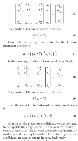
4. LP-ETAM Method
According to linear prediction theory, the delayed sample points in the time domain correspond to the array sensors in the spatial domain. For theM-sensor uniform line array, the p-order forward prediction filter in the spatial domain uses the data of the firstpsensors to estimate the data of the (p+ 1)th sensor, while thep-order backward prediction filter in the spatial domain uses the data of the last p sensors to estimate the data of the sensor before them.
Assume the data vector for the L snapshots of the ith sensor asXi =[xi(1) xi(2) . . . xi(L)] then the p-order forward prediction filter is
⎡ ⎢ ⎢ ⎢ ⎢ ⎢ ⎢ ⎢ ⎣ XT
p XpT−1 . . . X1T
XpT+1 XpT . . . X2T ..
. ... . .. ...
XMT−1 XMT−2 . . . XpT ⎤ ⎥ ⎥ ⎥ ⎥ ⎥ ⎥ ⎥ ⎦ ⎡ ⎢ ⎢ ⎢ ⎢ ⎢ ⎢ ⎢ ⎣ a1 a2 .. . ap ⎤ ⎥ ⎥ ⎥ ⎥ ⎥ ⎥ ⎥ ⎦ = ⎡ ⎢ ⎢ ⎢ ⎢ ⎢ ⎢ ⎣ XT p+1 XT p+2 XT M ⎤ ⎥ ⎥ ⎥ ⎥ ⎥ ⎥ ⎦ . (15)
The equation (15) can be written in short as
XT
faf =XTf0. (16) From (16) we can get the vector for the forward prediction coefficients
af =
XfXHf −1
XfXHf0 ∗
. (17)
In the same way,p-order backward prediction filter is ⎡ ⎢ ⎢ ⎢ ⎢ ⎢ ⎢ ⎢ ⎣
XpT+1 XTp+2 . . . XMT
XT
p XTp+1 . . . XMT−1 ..
. ... . .. ...
XT
2 X3T . . . XpT+1 ⎤ ⎥ ⎥ ⎥ ⎥ ⎥ ⎥ ⎥ ⎦ ⎡ ⎢ ⎢ ⎢ ⎢ ⎢ ⎢ ⎢ ⎣ b1 b2 .. . bp ⎤ ⎥ ⎥ ⎥ ⎥ ⎥ ⎥ ⎥ ⎦ = ⎡ ⎢ ⎢ ⎢ ⎢ ⎢ ⎢ ⎣ XT p XT p−1
X1T ⎤ ⎥ ⎥ ⎥ ⎥ ⎥ ⎥ ⎦ . (18)
The equation (18) can be written in short as
XT
bab=Xb0T. (19) Then the vector for the backward prediction coefficients is
ab=
XbXbH −1
XbXb0H ∗
. (20)
After we get the prediction coefficients, we can use them to extrapolate the array sensors. The array is extended as a sensor at one time. The forward prediction coefficients are used to extend the array forwardly. The backward prediction coefficients are used to extend the array backwardly.
The formula for forward prediction is
xk= p
i=1
aixk−i, k > M, (21)
whereaiis the forward prediction coefficient appearing in (15).
Similarly, the formula for backward prediction is
xk= p
i=1
bixk+i, k <1, (22)
wherebiis the backward prediction coefficient appearing in (18).
ap · · · a2 a1
+ xk
xk−p · · · xk−2 xk−1
Figure1: Schematic map for forward prediction filter.
abovementioned linear prediction technique is applied to the synthetic array obtained by ETAM method to further enlarge the aperture size, which results in improved performance over ETAM method.
Now we summarize the steps of the proposed LP-ETAM method in the following.
(1) To extend the M-sensor physical array to (M +
Jq)-sensor synthetic array by conventional ETAM method.
(2) To determine the prediction filter order p, calculate the forward and backward prediction coefficients according to (17) and (20).
(3) To extend the (M + Jq)-sensor synthetic array to (M+Jq+ 2K)-sensor virtual array by forward and backward prediction filter. In this process,Ksensors are extrapolated to the left and right of the synthetic array, respectively.
(4) To get the bearing estimation of targets by applying conventional beamforming technique to the virtual array obtained in step 3. Notice that the dimension of the steering vector is (M+Jq+ 2K)×1.
Figure 2gives the array aperture extension process in the proposed LP-ETAM method.
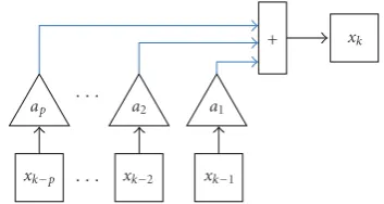
5. Performance Analysis
5.1. Angular Resolution. The performance of the LP-ETAM method has been tested with synthetic data; the relevant results are presented in this section. The far-field acoustic pressure measurements of a towed array have been simulated according to (1). In the numerical experiment, an 8-hydrophone towed array is considered with 1 m spacing moving with 5-knot speed. The received signal is assumed to be a narrow-band CW at 330 Hz. TheSNRat the hydrophone is −5 dB. In our simulations, the performance of the LP-ETAM method is compared with conventional beamforming method (CBF) and ETAM method. The integration time used to synthesize the aperture is 24 s, and the 8-hydrophone towed array is extended to a 64-hydrophone synthetic aperture by ETAM and a 192-hydrophone virtual aperture by LP-ETAM. The values of other parameters areq =M/2,
p=(M+Jq)/3, andK=M+Jq.
Figure 3 shows the directivity power patterns of the beamformer output for the three different methods when
Array moving direction θk
M-sensor physical array
Jextensions are made,q sensors are extended each time .
. .
(M+Jq)-sensor synthetic array obtained by ETAM .
.
. Kextensions are made , 2 sensors are extended to the array ends
each time
The final (M+Jq+ 2K)-sensor virtual array obtained by using linear prediction technique on the
synthetic array above. (1)
(2)
(3)
Figure2: The array aperture extension process.
there is a single source with bearings at 0◦. It is obvious that the mainlobe of LP-ETAM is much narrower than that of ETAM and CBF, indicating that LP-ETAM has the best angular resolution ability.
Figure 4 shows the directivity power patterns of the beamformer output for the three different methods when there are two widely spaced sources with bearings at −3◦ and 3◦.We notice that CBF cannot resolve the two sources but both LP-ETAM and ETAM can resolve them. Though both LP-ETAM and ETAM can resolve the two sources, the detection threshold for LP-ETAM is much lower than that of ETAM. This is easily deduced from the fact that the valley between the two source directions for LP-ETAM is deeper than the valley between the two source directions for ETAM.
Figure 5 shows similarly the directivity power patterns when there are two closely spaced sources with bearings at −1◦ and 1◦.We notice that both CBF and ETAM cannot resolve the two sources while LP-ETAM can resolve them, which means that LP-ETAM is superior to the other methods in angular resolution.
Figure 6 compares the probability of resolution for ETAM and LP-ETAM according to various SNRs. Two sources with azimuthsθ1andθ2are considered successfully “resolved” if both |θ1 − θ1| and |θ2 − θ2| are less than |θ1−θ2|/2, whereθ1is the estimate ofθ1andθ2is the estimate ofθ2. If two sources are successfully resolvedntimes inN
−20 −15 −10 −5 0 5 10 15 20 Azimuth (deg)
−10
−9
−8
−7
−6
−5
−4
−3
−2
−1 0
N
o
rm
alised
amplitude
(dB)
CBF ETAM LP-ETAM
Figure 3: The comparison of spatial spectrums of the three methods for a single source.
−20 −15 −10 −5 0 5 10 15 20
Azimuth (deg)
−8
−7
−6
−5
−4
−3
−2
−1 0
N
o
rm
alised
amplitude
(dB)
CBF ETAM LP-ETAM
Figure 4: The comparison of spatial spectrums of the three methods for two widely spaced sources.
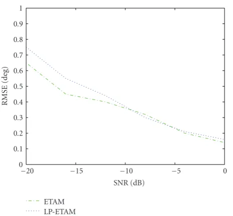
Figure 7 shows the root mean squared errors (RMSE) of ETAM and LP-ETAM according to various SNRs. The simulation conditions are the same as those used forFigure 6. It can be seen that the proposed LP-ETAM method does not produce better RMSE result. It is easy to under-stand since the proposed method is based on ETAM that the linear prediction technique helps extend the aperture but contributes little to reduce the bearing estimation variance.
−20 −15 −10 −5 0 5 10 15 20
Azimuth (deg)
−8
−7
−6
−5
−4
−3
−2
−1 0
N
o
rm
alised
amplitude
(dB)
CBF ETAM LP-ETAM
Figure 5: The comparison of spatial spectrums of the three methods for two closely-spaced sources.
−20 −15 −10 −5 0
SNR (dB) 0
10 20 30 40 50 60 70 80 90 100
P
robabilit
y
o
f
resol
ution
(%)
ETAM LP-ETAM
Figure6: The probability of resolution for ETAM and LP-ETAM.
5.2. Array Gain. In order to discuss array gain, we first define cross-correlation coefficients between differ-ent hydrophones. For a frequency band Δf with central frequency f0, the normalized cross-correlation coefficient
between thenth andmth hydrophones is defined as [9]
ρnm
f0
=
Q l=1Xn
fl
Xm∗
fl
Q
l=1Xn
fl2 Q
l=1Xm
fl2
, (23)
where fl,l = 1, 2,. . .,Q, are the frequency bins in the band
−20 −15 −10 −5 0 SNR (dB)
0 0.1 0.2 0.3 0.4 0.5 0.6 0.7 0.8 0.9 1
RMSE
(deg)
ETAM LP-ETAM
Figure7: The RMSE for ETAM and LP-ETAM.
parameter. When the noise field is white and isotropic, array gain is expressed as
G=10 log M
n=1 M
m=1ρnm
f0
M , (24)
whereMis the number of hydrophones in the physical array or extended array.
Figure 8presents the normalized cross-correlation coef-ficientsρnm(n=1, 2,. . ., 64, m=1, 2,. . ., 64) for the ETAM results of Figure 5 for the 100 Hz band in the frequency range 280–380 Hz with central frequency 330 Hz, which is the frequency of the two CW sources. The value of each coefficient is expressed as a circle in figure. The results in
Figure 8provide a quantitative estimate of the effectiveness of the extended aperture. Since the magnitude values of the coefficients are close to unity, it is apparent that the 64-hydrophone extended aperture is equivalent to a fully populated physical array.
Figure 9presents the normalized cross-correlation coef-ficients ρnm (n = 1, 2,. . ., 192, m = 1, 2,. . ., 192) for the LP-ETAM results ofFigure 5. We can see that the values are still close to unity even if the array aperture has been further extended, indicating the degree of coherence of the phase information related to the bearings of the sources across the extended apertures
The next step is to calculate the array gain for the physical and the synthetic apertures by using (24) and the values of the coefficientsρnmshown in Figures8and9. The expected array gain estimates for an 8-hydrophone, a 64-hydrophone, and a 192-hydrophone physical arrays are 9 dB, 18 dB, and 22.8 dB, respectively. The experimental array gain estimates for the 8-hydrophone physical array, the 64-hydrophone and the 192-hydrophone extended aperture are 6.9 dB, 15.8 dB, and 20.6 dB, respectively.
0 10 20 30 40 50 60
|n−m|
0 0.2 0.4 0.6 0.8 1 1.2
ρnm
Figure8: The normalized cross-correlation coefficients of the 64-hydrophone synthesized aperture.
0 20 40 60 80 100 120 140 160 180
|n−m|
0 0.2 0.4 0.6 0.8 1 1.2
ρnm
Figure9: The normalized cross-correlation coefficients of the 192-hydrophone synthesized aperture.
6. Lake Experiments
The lake experiment was designed to evaluate the angular resolution provided by the LP-ETAM method and the ETAM method in comparison with that provided by the physical array.
−100 −50 0 50 100 Azimuth (deg)
−45
−40
−35
−30
−25
−20
−15
−10
−5 0
N
o
rm
alised
amplitude
(dB)
CBF ETAM LP-ETAM
Figure 10: The comparison of spatial spectrums of the three methods (lake test result).
Results from the application of the LP-ETAM on the 8-hydrophone towed array for a 24-second observation period are shown inFigure 10. Hamming shading is adopted in each method prior to beamforming. The bearing estimates from the LP-ETAM method, shown by the dotted line inFigure 10, indicate the presence of the two expected sources while CBF and ETAM fail. This demonstrates the effectiveness of the proposed LP-ETAM method to provide improved angular resolution with respect to that provided by CBF and ETAM.
7. Conclusion
This paper focuses on the development of a new passive synthetic aperture technique that explores the merits of both linear prediction technique and ETAM method. The pro-posed LP-ETAM method employs spatial linear prediction technique to do extrapolation on the synthetic aperture obtained by ETAM to further enlarge the aperture size, which leads to superior angular resolution to conventional ETAM method. Simulation analysis shows that the proposed LP-ETAM method yields narrower beams and higher array gain than ETAM method. Results from application of ETAM method and the proposed LP-ETAM method on real data with very stable CW signals have shown that the angular resolution provided by LP-ETAM resolves two closely spaced sources that are unresolvable by the ETAM method.
Acknowledgment
This work was supported by the National Natural Science Foundation of China (60972152), Aeronautical Science Foundation of China (2009ZC53031), and the Basic Research Foundation of Northwestern Polytechnical University (NPU-FFR-W018102).
References
[1] N.-C. Yen and W. Carey, “Application of synthetic-aperture processing to towed-array data,” Journal of the Acoustical Society of America, vol. 86, no. 2, pp. 754–765, 1989.
[2] S. Stergiopoulos, “Extended towed array processing by an overlap correlator,”Journal of the Acoustical Society of America, vol. 86, no. 1, pp. 158–171, 1989.
[3] A. H. Nuttall, “The maximum likelihood estimator for acous-tic syntheacous-tic aperture processing,” IEEE Journal of Oceanic Engineering, vol. 17, no. 1, pp. 26–29, 1992.
[4] S. Stergiopoulos and H. Urban, “A new passive synthetic aperture technique for towed arrays,”IEEE Journal of Oceanic Engineering, vol. 17, no. 1, pp. 16–25, 1992.
[5] G. S. Edelson and D. W. Tufts, “On the ability to estimate narrow-band signal parameters using towed arrays,” IEEE Journal of Oceanic Engineering, vol. 17, no. 1, pp. 48–61, 1992. [6] R. Rajagopal and P. R. Rao, “Performance comparison of PASA beamforming algorithms,” inProceedings of the International Symposium on Signal Processing and Its Applications (ISSPA ’96), vol. 2, pp. 825–828, Gold Coast, Australia, August 1996. [7] R. Rajagopal and P. R. Rao, “Modified extended towed array
method (METAM) for passive synthetic aperture beamform-ing,” inProceedings of the International Symposium on Signal Processing and Its Applications (ISSPA ’96), vol. 2, pp. 772–775, Gold Coast, Australia, August 1996.
[8] S. Kim, D. H. Youn, and C. Lee, “Temporal domain processing for a synthetic aperture array,” IEEE Journal of Oceanic Engineering, vol. 27, no. 2, pp. 322–327, 2002.
[9] S. Stergiopoulos and H. Urban, “An experimental study in forming a long synthetic aperture at sea,” IEEE Journal of Oceanic Engineering, vol. 17, no. 1, pp. 62–72, 1992.
[10] Z. G. Zhang, S. C. Chan, and K. M. Tsui, “A recursive frequency estimator using linear prediction and a Kalman-filter-based iterative algorithm,”IEEE Transactions on Circuits and Systems II, vol. 55, no. 6, pp. 576–580, 2008.