Volume 2010, Article ID 596842,10pages doi:10.1155/2010/596842
Research Article
Facial Affect Recognition Using Regularized Discriminant
Analysis-Based Algorithms
Chien-Cheng Lee, Shin-Sheng Huang, and Cheng-Yuan Shih
Department of Communications Engineering, Yuan Ze University, 135 Yuan-Tung Road, Chung-Li, Taoyuan County 320, Taiwan
Correspondence should be addressed to Chien-Cheng Lee,[email protected]
Received 3 December 2009; Accepted 17 February 2010
Academic Editor: Jenq-Neng Hwang
Copyright © 2010 Chien-Cheng Lee et al. This is an open access article distributed under the Creative Commons Attribution License, which permits unrestricted use, distribution, and reproduction in any medium, provided the original work is properly cited.
This paper presents a novel and effective method for facial expression recognition including happiness, disgust, fear, anger, sadness, surprise, and neutral state. The proposed method utilizes a regularized discriminant analysis-based boosting algorithm (RDAB) with effective Gabor features to recognize the facial expressions. Entropy criterion is applied to select the effective Gabor feature which is a subset of informative and nonredundant Gabor features. The proposed RDAB algorithm uses RDA as a learner in the boosting algorithm. The RDA combines strengths of linear discriminant analysis (LDA) and quadratic discriminant analysis (QDA). It solves the small sample size and ill-posed problems suffered from QDA and LDA through a regularization technique. Additionally, this study uses the particle swarm optimization (PSO) algorithm to estimate optimal parameters in RDA. Experiment results demonstrate that our approach can accurately and robustly recognize facial expressions.
1. Introduction
Human-computer interaction (HCI) technologies have attracted more and more attention. The traditional interface devices such as the keyboard and mouse are constructed to transmit explicit messages. The implicit information about the user, such as changes in the affective state, is ignored. However, HCI is moving gradually from computer-centered designs toward human-computer-centered designs [1, 2]. Designs for human-centered computing should focus on the human portion of the HCI context, like nonlinguistic conversational signal, emotion, and affective states. Human-centered interfaces must have the ability to detect human affective behavior because it conveys fundamental com-ponents of human-human communication. These affective states motivate human actions and enrich the meaning of human communication.
Previous research [3] shows that 55% of face-to-face human communication is relied on facial expressions, indicating that facial expressions play an important role in social interactions between human beings. As a result, facial expressions are also an important part of HCI. Thus,
automatic facial expression recognition in the human-computer environment is an essential and challenging task.
Various techniques have been developed for automatic facial expression recognition. Three recent surveys [4–7] on this topic indicate that facial expression recognition has grown more sophisticated. Facial expression recognition techniques can be categorized based on recognition targets or data sources. With respect to recognition targets, most techniques attempt to recognize a small set of prototypic emotional expressions, that is, happiness, surprise, anger, sadness, fear, and disgust, as well as the neutral state. This practice is based on the work of Darwin [8] and more recently Keltner and Ekman [9] who proposed that basic emotions have corresponding prototypic facial expressions. Ekman and Friesen [10] developed the Facial Action Coding System (FACS) for describing facial expressions in terms of action units (AUs). FACS consists of 46 AUs, which describe basic facial movements based on muscle activities. Various researchers engage in AUs recognition to model facial actions [11].
images and image sequences. In sequence-based methods, an image sequence displays one expression. Thus, a neutral face must be identified first to serve as a baseline face. Then, expression recognition depends on the difference between the baseline face and the following input face image. Optical flow estimation is a typical method of extracting facial features. Yacoob and Davis [12] used the optical flow approach to track the motion of facial features from image sequences and classified the extracted facial features into six basic expressions. Bartlett et al. [13] used a method combining principal component analysis (PCA) with optical flow for facial expression recognition. Essa and Pentland [14] used optical flow in a physical model of the face with a recursive framework to classify facial expressions. Xiang et al. [15] used Fourier transform to extract facial features and represent expressions. These features are then processed using fuzzy C means clustering to generate a spatiotemporal model for each expression type.
If the baseline image in the sequence-based methods is not identified correctly, it is difficult to identify the facial expression for a given image frame. However, facial expression recognition using static images is more difficult than that using image sequences because less information is available. Psychologists often use single images for expression recognition. Therefore, facial expression recognition using static images has attracted a lot of attention. Chen and Huang [16] proposed a clustering-based feature extraction method for facial expression recognition. They used the AR database, created by Aleix Martinez and Robert Benavente, to classify three facial expressions: neutral, smiling, and angry. Zhi and Ruan [17] proposed a method called the two-dimensional discriminant locality preserving projections (2D-DLPPs) algorithm and applied the method to facial expression recognition in a Japanese female facial expression database (JAFFE) and the Cohn-Kanade database. Shin et al. [18] combined the two-dimensional learning discriminant analysis (2D-LDA) and support vector machine (SVM) methods to recognize seven basic expressions. Feng et al. [19] divided face images into small regions and extracted local binary pattern (LBP) histograms as features and then used a linear programming technique to classify seven facial expressions.
This paper proposes a novel regularized discriminant analysis-based boosting algorithm (RDAB) to recognize seven expressions, including happiness, surprise, anger, sadness, fear, disgust, and a neutral state, from static images. The proposed method also employs an entropy criterion to select effective Gabor features for facial image representation which is a subset of informative and non-redundant Gabor features. In RDAB, regularized discriminant analysis (RDA) acts as a learner in the boosting algorithm. RDA combines the strengths of linear discriminant analysis (LDA) and quadratic discriminant analysis (QDA) and solves the small sample size and ill-posed problems of QDA and LDA by regularizing parameters. This study also uses a particle swarm optimization (PSO) algorithm to estimate the opti-mal parameters in RDA. Experiment results demonstrate that the proposed RDAB facial expression method achieves a high
recognition rate and outperforms other facial expression recognition systems.
The rest of this paper is organized as follows.Section 2 provides an overview of the proposed method. Section 3 describes each component of the proposed method. Section 4 presents experiment results. Finally, conclusions are summarized inSection 5.
2. Overview of the Proposed Method
The overall process of the proposed facial expression recogni-tion method is displayed inFigure 1. First, the preprocessing step is applied to input images to produce standardized facial images for subsequent processing. Facial images are detected using the Viola and Jones face detector [20]. The original images are cropped into face images and resized to 128 ×
96. Then, a histogram equalization method is applied to eliminate variations in illumination. Several previous studies [21] show that classification using downsampled images in pattern recognition produces a higher accuracy than using the original images. Using downsampled images also reduces the computation complexity. Thus, the following feature extraction step uses facial images that have been downsampled by a factor of two.
Automated facial expression recognition must solve two basic problems: facial feature extraction and facial expression classification. Facial feature extraction methods can be cate-gorized in terms of image sequences or static images. Motion extraction approaches directly focus on facial changes that occur due to facial expressions, whereas static image-based methods do not rely on neutral face images to extract facial features. Gabor features are widely used in image analysis because they closely model the receptive field properties of cells in the primary visual cortex [22–24]. Therefore, this study uses Gabor features to recognize facial expressions from static images.
In practice, the dimensionality of a Gabor feature vector is so high that the computation and memory requirements are very large. For example, if an image measures 128 ×
96 pixels, the dimensionality of the Gabor feature vector with three frequencies and eight orientations is 294912 (128×
96×3×8). Some of these features are similar. In other words, using the Gabor features with all frequencies and orientations is redundant. For this reason, several sampling methods have been proposed to determine the “optimal” subset for extracting Gabor features. Liu et al. [25] proposed an optimal sampling of Gabor features using PCA for face recognition. Additionally, AdaBoost has been widely used for feature selection [26–28]. This study proposes an effective Gabor feature selection to extract the informative Gabor features representing the facial characteristics. Entropy is used as a criterion to measure the importance of the feature. This approach reduces the feature dimensionality without losing much information and also decreases computation and storage requirements.
vector machines (SVMs), and boosting algorithms. SVMs and boosting algorithms are both large margin classifiers primarily designed for two-class classification problems. SVMs often adopt one strategy or one-against-all procedure to deal with multiclass problems. On the other hand, boosting algorithms can solve multiclass problems using a multiclass learner. Thus, several researchers have used boosting algorithms with different learners to process multiclass problems. Yang et al.[29] adopted the AdaBoost algorithm to learn the combination of optimal discrimi-native features to construct the classifier and classify seven expressions and several AUs. Lu et al. [30] developed a novel boosting algorithm combined with LDA-based learners for face recognition. This paper proposes an RDA-based boosting algorithm to recognize facial expressions. RDA combines the benefits of LDA and QDA to achieve a higher recognition rate.
3. Automatic Facial Expression
Recognition System
The block diagram of the automatic facial expression recog-nition system is shown inFigure 1. The key components of the proposed approach include (1) preprocessing, (2) eff ec-tive Gabor feature selection, and (3) RDAB classification. The details of proposed method are described as follows.
3.1. Preprocessing. This preprocessing is an important step because the input images usually have some slight diff er-ences, such as head tilt and head size. The preprocessing phase takes the segmented face, normalizes the face images, reduce lighting variations, and downsamples the face images. The preprocessing phase contains the following steps.
(1) It detects faces from input images.
(2) It normalizes the face regions with respect to a 128×
96 face image by using the eyes and nose as reference points.
(3) It performs histogram equalization to reduce the nonuniformity in the pixel distributions that may occur due to various imaging situations.
(4) It downsamples the face images to obtain the low-frequency images. In this way, the noise and the computation complexity will be reduced.
3.2. Effective Gabor Feature Extraction. The Gabor filter is a very useful tool in computer vision and image analysis because it has optimal localization properties in both spatial and frequency analysis. A 2D Gabor filter is a complex field sinusoidal grating modulated by a 2D Gaussian function in the spatial domain. The 2D Gabor filterG(x,y) is defined as
hx,y=gx,y·expi2πUx+V y, (1)
where (x,y) = (xcosφ + ysinφ,−xsinφ + ycosφ) are rotated coordinates, in which the major axis is oriented at
an angleφfrom thex-axis, (U,V) represents a particular 2D frequency, and
gx,y= 1
2πλσxσy exp
⎧ ⎨ ⎩−12
⎡ ⎣x/η
σx
2
+
y σy
2⎤ ⎦ ⎫ ⎬
⎭, (2)
whereσxandσyrepresent the spatial extent and bandwidth of the filter, andηis the aspect ratio betweenxandyaxes. For convenience, we assume thatσx = σy = σ, the aspect ratio isη =1, and thex-axis of the Gaussian has the same orientation as the frequency; hence, (1) can be simplified to
hx,y=gx,y·exp[i2πFx], (3)
whereF=√U2+V2is called the modulation frequency.
This study considers a class of self-similar functions called Gabor wavelets. Using (3) as the mother Gabor wavelet, the self-similar filter bank can be derived by dilations and rotations ofh(x,y) through the generating function:
hmn
x,y=β−mhx,y,
β >1, m=1, 2,. . .,S, n=1, 2,. . .,T, (4)
wherex=β−m(xcosφ
n+ysinφn),y =β−m(−xsinφn+ ycosφn), and φn = π(n− 1)/T. The subscripts m and
n represent the index for scale (dilation) and orientation (rotation).Sis the total number of scales andTis the total number of orientations.
For a given input image I(x,y), the magnitude of a filtered imageFmn(x,y) can be obtained as
Fmn
x,y
=hRmn(x,y)∗I(x,y)2+hImn(x,y)∗I(x,y)2, (5)
where ∗ indicates 2-D convolution, and hRmn(x,y) and hImn(x,y) represent the real and imaginary parts of the Gabor filters from (4). The real part of Gabor filters with three scales and eight orientations is shown inFigure 2.
Entropy is a measure of the uncertainty associated with a random variableXin information theory, defined as
H(X)= −
x
p(X=x) logp(X=x). (6)
The less uncertainty there is, the less entropy there is. Conversely, more uncertainty produces more entropy. The objective of feature selection is to select a subset of features that gives as much information as possible. Thus, this study formulates an effective feature selection scheme based on the feature position probability distribution to select the informative Gabor features. Let Om,n,x,y(r) denote the
occurrence of Gabor magnitude response r in Fmn(x,y) for all training images. The feature position probability is defined as
pm,n,x,y(r)=
Om,n,x,y(r)
nL
Preprocessing Input
images
Effective Gabor feature selection
RDAB classification
Facial Expression
Figure1: Overall process of the proposed facial expression recognition method.
Figure2: The real part of the Gabor filters with three scales and eight orientations.
where
nL= L
r=0
Om,n,x,y(r), for 0≤r≤L. (8)
The entropy of the feature position probability distribution is defined as
Hm,n,x,y(R)= −
r
pm,n,x,y(R=r) log
pm,n,x,y(R=r)
,
(9)
where R is a random variable of the occurrence of Gabor magnitude response. The value of the entropy Hm,n,x,y(R)
indicates that the uncertainty of the feature at the pixel position (x,y) of the Gabor features with mth scale and
nth orientation for all training images. A larger value of Hm,n,x,y(R) means that the feature magnitudes vary from
different images. Thus, features along this range of the feature space can improve the discriminating power between different expression classes. On the other hand, a smaller value of the entropyHm,n,x,y(R) indicates the corresponding
features tend toward the same magnitude. That is, features along this range contribute less to discrimination. To reduce the feature space, these features should not be considered in the classification phase. Accordingly, sort Hm,n,x,y(R) in
descending order and use the firstM≤NGabor features as the feature vector to form a lowerM-dimensional subspace, whereN is the dimensionality of the original feature space andMis that of the effective feature space.Figure 3shows an example of effective Gabor filters of a face image with three scales and eight orientations. Figure 3(a) shows the magnitudes of the Gabor features. Figure 3(b) shows the points of the top 10 percent of the Gabor features.
3.3. RDA-Based Boosting Algorithm. RDA combines the
strengths of LDA and QDA, offering several advantages
compared to the conventional LDA and QDA. LDA and QDA are well known and popular methods in classification and recognition. However, these approaches often suffer from the small sample size problem (SSS) that exists in high-dimensional pattern recognition tasks. To solve the SSS problem, the traditional solution adopts a two-phase framework PCA plus LDA for feature compression and selection. However, the PCA may discard dimensions that contain important discriminative information [31]. Thus RDA, an intermediate method between LDA and QDA, is proposed to deal with this problem [32].
3.3.1. Regularized Discriminant Analysis. Given a set of objectsZ, the purpose of classification or discriminant is to assign objects to one of severalK classes. The classification rule is based on a quantity called the discriminant score for thekth class, defined as
dk=1min≤k≤Kdk(Z), (10)
with
dk(Z)=
Z−μk
T Σ−1
k
Z−μk
+ ln|Σk| −2 lnπk, (11)
wherekdenotes thekth class, andμk andΣkare mean and covariance matrix of thekth class, respectively. In the case of LDA, variables are normally distributed in each class with different mean vectors and a common covariance matrix. On the other hand, the variables in QDA are assumed to be normally distributed in each class with different mean vectors and different covariance matrices.
(a)
(b)
Figure3: Example of the effective Gabor filter of a face image with three scales and eight orientations. (a) Original Gabor features. (b) Points of the top ten percent of the Gabor features (white points).
covariance matrices. Hence, classification based on QDA requires larger samples than those based on LDA. Addi-tionally, in small-sample classification, reducing the number of estimated parameters by using the pooled covariance estimate may lead to superior performance, even if the class covariance matrices are substantially different. That is, LDA generally outperforms QDA in SSS problems. For these reasons, RDA provides a regularization mechanism to shrink the separate covariance of QDA toward a common
covariance as in LDA. The regularized covariance matrix of
kth class is
Σk(λ)=λSw+ (1−λ)Σk, (12)
γ (0, 1) (1, 1)
LDA QDA
Weighted nearest-means
Nearest-means
(0, 0) (1, 0) λ
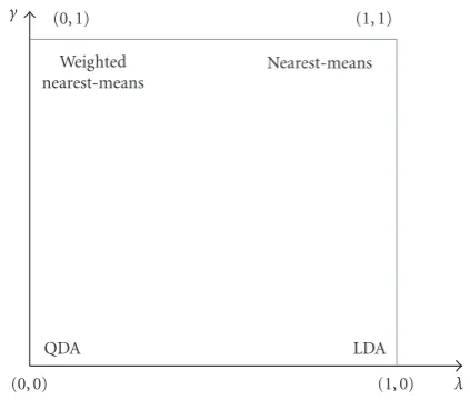
Figure4: RDA model selection. (λ=0, γ =0) represents QDA, (λ=1,γ=0) represents LDA, (λ=1, γ=1) corresponds to the nearest-means classifier, and (λ=0, γ=1) represents a weighted nearest-means classifier.
n, is less than the data dimensionality, QDA and LDA are ill-posed. Additionally, biasing the class covariance matrices toward commonality may not be an effective shrinkage way. According to [33], ridge regression regularizes ordinary linear least squares regression by shrinking toward a multiple of the identity matrix. Therefore, the regularization should be
Σkλ,γ=1−γΣk(λ) +γ
dtrace[Σk(λ)]Id, (13)
where Id is an identity matrix of size d by d andd is the dimensionality of the data. The termsλandγrepresent two parameters that range from 0 to 1.
RDA provides a fairly rich class of regularization alterna-tives.Figure 4shows four corners in the (λ,γ) plane repre-senting well-known classification procedures. The lower left corner (λ = 0, γ = 0) represents QDA. The lower right (λ = 1, γ = 0) represents LDA. The upper right corner (λ= 1, γ =1) corresponds to the nearest-means classifier. The upper left corner of the plane represents a weighted nearest-means classifier.
3.3.2. Model Selection. A good pair of values forλandγis not likely to be known in advance. Selecting an optimal value for a parameter pair such as (λ,γ) is calledmodel selection. Because model selection is a type of optimization problem, this study uses a PSO algorithm [34] to obtain the optimal parameters. The basic concept of PSO algorithm is described as follows.
Suppose that theith particle of the swarm is denoted byXi = (xi1,xi2,. . .,xid), and the velocity vector of the ith
particle is denoted byVi =(vi1,vi2,. . .,vid). Equations (14)
shows the particle position and the velocity vector updating:
Vi=Vi+c1rand( )(Pi−Xi) +c2rand( )
Pg−Xi
,
Xi=Xi+Vi,
(14)
where rand( ) is a random number generated within (0,1). The termsc1andc2 are positive constant parameters which
control the maximum step size. Pi = (pi1,pi2,. . .,pid)
is the best solution achieved so far by Xi particle, and Pg = (pg1,pg2,. . .,pgd) is the best solution achieved so far
for the whole particles. The velocity vector Vi is confined within [Vmin,Vmax], and it is set equal to the corresponding
threshold if the velocity vector exceeds the thresholdVminor
Vmax. The PSO procedure is given as follows.
(1) Randomly initializeXiandViof all particles. (2) Evaluate the fitness values of all particles, and update
PiandPg.
(3) UpdateXiandViaccording to (14).
(4) Evaluate the fitness values of all particles, and update PiandPg.
(5) If the convergence condition is not reached, go back to step (3).
3.3.3. Boosting Procedure. The ability of a boosting algorithm to reduce the overfitting and generalization errors of clas-sification problems is quite interesting. In the traditional AdaBoost algorithm, the learner is weak and just slightly better than random guessing. In contrast, the proposed RDA-based boosting algorithm uses Direct LDA (DLDA) [35] to reduce dimensionality and extract discriminative features. RDA then performs the classification tasks.
Algorithm 1 illustrates the proposed RDA-based boost-ing algorithm. Given a trainboost-ing setX = {Xi}ci=1, containing
Cclasses, each classXi= {(xi j,yi j)}Lij=1consists of a number
of examplesxi jand their corresponding class labelsyi j.N=
C
i=1Liis the total number of examples in the set. LetXbe the sample space:xi j ∈Xand atY= {1,. . .,C}be the label set: yi j ∈ Y. The goal of learning is to estimate a classifier h(x) : X → Y, which will correctly classify unseen examples. It works by repeatedly applying a given learner to a weighted version of the training set in T iterations and combining these learners{ht}t=1,...,Tat each iteration into a single strong classifier.
4. Experiment Results
(1) Given set of training imagesX= {(xi j,yi j)Lj=i1}Ci=1with labelsyi j=i∈Y, whereY= {1,. . .,C};
a DLDA feature extractor and an RDA-based learner; and the iteration number,T. LetB= {(xi j,y) : xi j∈X, y∈Y, y /∈yi j}
(2) Initialized1(xi j,y)=1/|B| =1/N(C−1), the mislabel distribution overB.
(3) Fort=1,. . .,T, repeat the following steps:
(a) Update the pseudo sample distribution:Dt(xi j)=
y /=yi jdt(xi j,y)
(b) If t=1: randomly choosensamples per class to form a learning setR1⊂X (c) else: choosenhardest samples per class based onDtto formRt⊂X
(d) Train a DLDA feature extractorP, which is a projection matrix, to obtain discriminative feature set (ψt,{xi,t}Ci=1) (e) Use PSO to find the optimal parameters (λ,γ) of covariance matrix in RDA.
(f) Build an RDA learnerht=r(ψt,{xi,t}Ci=1), apply it into the entire training setX,and normalize the classified result from 0 to 1 by (rmax−rx,i)/(rmax−rmin).
(g) Calculate the pseudo-loss produced byht:εt=(1/2)(xi j,y)∈Bdt(xi j,y)(1−ht(xi j,yi j) +ht(xi j,y)).
(h) Setβt=εt/(1−εt). Ifβt=0, thenT=t−1 and abort loop.
(i) Update the mislabel distributiondt:dt+1(xi j,y)=dt(xi j,y)·βt(1+ht(xi j,yi j)+ht(xi j,y))/2
(j) Normalizeγt+1so that it is a distribution,dt+1(xi j,y)←dt+1(xi j,y)/
(xi j,y)∈Bdt+1(xi j,y)
(4) Output the final composite classifierhf(x)=arg maxy∈Y
(log(1/βt))ht(x,y)
Algorithm1: RDA-based boosting algorithm.
twenty-nine segments per class are used to train and the remaining segment is used to test. The procedure of training and testing is repeated thirty times until each segment has been used in test. Finally, all the recognition rates are averaged to obtain an overall recognition rate for the proposed method.
The performance of the proposed system can be affected by two factors. One is the effective Gabor feature selection and the other is the number of hardest-to-classify samples in RDAB algorithm.Table 1compares different levels of the effective Gabor features. Results show that the top ten percent of the selected Gabor features with three scales and eight orientations achieve the highest recognition rate of 96.67%. This means that there was a 10-fold reduction in the number of Gabor filters used. The results also clearly show that the Gabor features with three scales and eight orientations outperform those with five scales and eight orientations. In this experiment, the number of iterations in RDAB algorithm is 25. The number of hardest-to-classify images per class is 12.
The RDAB algorithm selects many hardest-to-classify samples to train the learner in each iteration. The number of hardest-to-classify samples affects the learner’s capacity. Consequently, the optimal number of hardest-to-classify samples can improve the classifier efficiency.Figure 6 com-pares the recognition rates for different numbers of hardest-to-classify samples. This figure shows that the highest recognition rate, 96.67%, is achieved when the number of hardest-to-classify is samples 12 for the top ten percent of the selected Gabor features with three scales and eight orientations. As the number of hardest-to-classify samples increases, the recognition rate decreases due to the overfitting problem. These results also indicate that Gabor features with three scales and eight orientations perform better than those with five scales and eight orientations. The number of iterations in RDAB algorithm in this experiment is 25, and the top ten percent of the selected Gabor features are used.
Table1: Recognition rates for different levels of the effective Gabor features.
Percentage of Selected Features
Recognition Rates 3 scales and 8
orientations
5 scales and 8 orientations
5 93.81% 90.95%
10 96.67% 92.38%
20 94.76% 93.81%
30 93.81% 94.76%
40 92.86% 93.81%
50 94.29% 92.86%
60 94.76% 92.38%
70 94.29% 92.38%
80 95.24% 92.38%
90 95.71% 92.38%
100 94.29% 92.38%
Table2: Comparison of facial expression recognition using JAFFE database.
Methods Recognition rates (%)
Zhi and Ruan [17] 95.91
Shin et al. [18] 95.71
Feng et al. [19] 93.8
Zhao et al. [36] 93.72
Qi and Jiang [37] 94.64
Liejun et al. [38] 95.7
Our proposed method 96.67
Figure5: Seven basic emotions (from left to right): anger, disgust, fear, happiness, sadness, surprise, and neutral state (images taken from JAFFE database).
Table3: Confusion matrix of facial expression recognition.
Anger Disgust Fear Happiness Sadness Surprise Neutral Total
Anger 30
Disgust 29 1
Fear 1 27 1 1
Happiness 30
Sadness 2 28
Surprise 29 1
Neutral 30
203/210
40 50 60 70 80 90 100
R
ec
o
ng
nition
rat
e
0 5 10 15 20 25 30 35
Number of hardest-to-classify samples 3 scales and 8 orientations
5 scales and 8 orientations
Figure6: A comparison of different numbers of hardest-to-classify samples.
image sequences. This study only compares experiments using JAFFE static images, asTable 2 shows. In [17], facial expression classification performance was tested on feature vectors derived from two-dimensional discriminant locality preserving projections, producing a 95.91% recognition rate. Shin et al. [18] investigated various feature representation and expression classification schemes to recognize seven different facial expressions. Their experiment results show that the method of combining 2D-LDA (Linear Discriminant
Analysis) and SVM outperforms other methods, producing a 95.71% recognition rate using the leave-one-out strategy. Feng et al. [19] reported an accuracy of 93.8% based on local binary pattern histograms and linear programming techniques. In [36], a method for facial expression recog-nition with Non-negative Matrix Factorization (NMF) and PCA-NMF is presented, and their best recognition rate is 93.72%. The work reported in [37,38] produced recognition rates of 94.64% and 95.7%, respectively. In this study, we use a leave-one-out strategy similar to that in [18] to verify our algorithm. Our recognition rate of 96.67% outperforms other methods tested on the same database.Table 3 shows the confusion matrix, indicating that anger, happiness, and the neutral state are recognized with very high accuracy, but other expressions (disgust, fear, sadness, surprise) are sometimes confused.
5. Conclusion
adopted to cope with the modal selection problem in RDA. The results of this study show that the proposed method has a high recognition rate of 96.67%, which is better than other reported results. The confusion matrix also shows that anger, happiness, and the neutral state are recognized with very high accuracy.
Acknowledgment
The authors would like to thank the National Science Council (Grant no. NSC 98-2221-E-155-050) for supporting this work.
References
[1] M. Pantic, A. Pentland, A. Nijholt, and T. Huang, “Human computing and machine understanding of human behavior: a survey,” inProceedings of the 8th International Conference on Multimodal Interfaces (ICMI ’06), pp. 239–248, 2006. [2] Z. Zeng, M. Pantic, G. I. Roisman, and T. S. Huang, “A
survey of affect recognition methods: audio, visual, and spon-taneous expressions,”IEEE Transactions on Pattern Analysis and Machine Intelligence, vol. 31, no. 1, pp. 39–58, 2009. [3] A. Mehrabian, “Communication without words,”Psychology
Today, vol. 2, no. 4, pp. 53–56, 1968.
[4] A. Samal and P. A. Iyengar, “Automatic recognition and analysis of human faces and facial expressions: a survey,” Pattern Recognition, vol. 25, no. 1, pp. 65–77, 1992.
[5] M. Pantic and L. J. M. Rothkrantz, “Automatic analysis of facial expressions: the state of the art,”IEEE Transactions on Pattern Analysis and Machine Intelligence, vol. 22, no. 12, pp. 1424– 1445, 2000.
[6] B. Fasel and J. Luettin, “Automatic facial expression analysis: a survey,”Pattern Recognition, vol. 36, no. 1, pp. 259–275, 2003. [7] M. Pantic and M. S. Bartlett, Machine Analysis of Facial
Expressions, Face Recognition, I-Tech Education and Publish-ing, 2007.
[8] C. Darwin,The Expression of Emotions in Man and Animals, John Murray, London, UK, 1965, reprinted by University of Chicago Press.
[9] D. Keltner and P. Ekman, “Facial expression of emotion,” in Handbook of Emotions, M. Lewis and J. M. Haviland-Jones, Eds., pp. 236–249, Guilford, New York, NY, USA, 2000. [10] P. Ekman and W. V. Friesen, The Facial Action Coding
System: A Technique for the Measurement of Facial Movement, Consulting Psychologists Press, 1978.
[11] G. Donato, M. S. Bartlett, J. C. Hager, P. Ekman, and T. J. Sejnowski, “Classifying facial actions,”IEEE Transactions on Pattern Analysis and Machine Intelligence, vol. 21, no. 10, pp. 974–989, 1999.
[12] Y. Yacoob and L. Davis, “Recognizing faces showing expres-sions,” inProceedings of the International Workshop on Auto-matic Face and Gesture Recognition, pp. 278–283, 1995. [13] M. S. Bartlett, J. C. Hager, P. Ekman, and T. J. Sejnowski,
“Measuring facial expressions by computer image analysis,” Psychophysiology, vol. 36, no. 2, pp. 253–263, 1999.
[14] I. A. Essa and A. P. Pentland, “Coding, analysis, interpretation, and recognition of facial expressions,”IEEE Transactions on Pattern Analysis and Machine Intelligence, vol. 19, no. 7, pp. 757–763, 1997.
[15] T. Xiang, M. K. H. Leung, and S. Y. Cho, “Expression recognition using fuzzy spatio-temporal modeling,” Pattern Recognition, vol. 41, no. 1, pp. 204–216, 2008.
[16] X. W. Chen and T. Huang, “Facial expression recognition: a clustering-based approach,”Pattern Recognition Letters, vol. 24, no. 9-10, pp. 1295–1302, 2003.
[17] R. Zhi and Q. Ruan, “Facial expression recognition based on two-dimensional discriminant locality preserving projec-tions,”Neurocomputing, vol. 71, no. 7–9, pp. 1730–1734, 2008. [18] F. Y. Shin, C. F. Chuang, and P. S. P. Wang, “Performance com-parisons of facial expression recognition in JAFFE database,” International Journal of Pattern Recognition and Artificial Intelligence, vol. 22, no. 3, pp. 445–459, 2008.
[19] X. Feng, M. Pietik¨ainen, and A. Hadid, “Facial expression recognition based on local binary patterns,”Pattern Recogni-tion and Image Analysis, vol. 17, no. 4, pp. 592–598, 2007. [20] P. Viola and M. Jones, “Rapid object detection using a
boosted cascade of simple features,” inProceedings of the IEEE Computer Society Conference on Computer Vision and Pattern Recognition, vol. 1, pp. 511–518, 2001.
[21] Y. Xu and Z. Jin, “Down-sampling face images and low-resolution face recognition,” inProceedings of the 3rd Inter-national Conference on Innovative Computing Information and Control (ICICIC ’08), p. 392, 2008.
[22] J. G. Daugman, “Complete discrete 2-D Gabor transforms by neural networks for image analysis and compression,”IEEE Transactions on Acoustics, Speech, and Signal Processing, vol. 36, no. 7, pp. 1169–1179, 1988.
[23] C. C. Tsai, J. Taur, and C. W. Tao, “Iris recognition based on relative variation analysis with feature selection,”Optical Engineering, vol. 47, no. 9, Article ID 097202, 2008.
[24] B. Zhang, Z. Wang, and B. Zhong, “Kernel learning of histogram of local Gabor phase patterns for face recognition,” EURASIP Journal on Advances in Signal Processing, vol. 2008, Article ID 469109, 8 pages, 2008.
[25] D. H. Liu, K. M. Lam, and L. S. Shen, “Optimal sampling of Gabor features for face recognition,”Pattern Recognition Letters, vol. 25, no. 2, pp. 267–276, 2004.
[26] G. Littlewort, M. S. Bartlett, I. Fasel, J. Susskind, and J. Movel-lan, “Dynamics of facial expression extracted automatically from video,”Image and Vision Computing, vol. 24, no. 6, pp. 615–625, 2006.
[27] L. Shen and L. Bai, “Information theory for Gabor feature selection for face recognition,”EURASIP Journal on Applied Signal Processing, vol. 2006, Article ID 30274, 11 pages, 2006. [28] L. Shen, L. Bai, D. Bardsley, and Y. Wang, “Gabor feature
selection for face recognition using improved AdaBoost learn-ing,” inProceedings of the International Wokshop on Biometric Recognition Systems (IWBRS ’05), vol. 3781 ofLecture Notes in Computer Science, pp. 39–49, Beijing, China, October 2005. [29] P. Yang, Q. Liu, and D. N. Metaxas, “Boosting encoded
dynamic features for facial expression recognition,” Pattern Recognition Letters, vol. 30, no. 2, pp. 132–139, 2009. [30] J. Lu, K. N. Plataniotis, A. N. Venetsanopoulos, and S. Z. Li,
“Ensemble-based discriminant learning with boosting for face recognition,”IEEE Transactions on Neural Networks, vol. 17, no. 1, pp. 166–178, 2006.
[32] J. H. Friedman, “Regularized discriminant analysis,”Journal of the American Statistical Association, vol. 84, no. 405, pp. 165– 175, 1989.
[33] A. Hoerl and R. Kennard, “Ridge regression: biased estimation for non-orthogonal problems,”Technometrics, vol. 12, no. 3, pp. 55–67, 1970.
[34] J. Kennedy and R. Eberhart, “Particle swarm optimization,” inProceedings of the IEEE International Conference on Neural Networks, vol. 4, pp. 1942–1948, 1995.
[35] H. Yu and J. Yang, “A direct LDA algorithm for high-dimensional data with application to face recognition,”Pattern Recognition, vol. 34, pp. 2067–2070, 2001.
[36] L. Zhao, G. Zhuang, and X. Xu, “Facial expression recognition based on PCA and NMF,” inProceedings of the World Congress on Intelligent Control and Automation (WCICA ’08), pp. 6822– 6825, 2008.
[37] X. X. Qi and W. Jiang, “Application of wavelet energy feature in facial expression recognition,” inProceedings of the IEEE International Workshop on Anti-Counterfeiting, Security, Identification (ASID ’07), pp. 169–174, 2007.