Volume 2010, Article ID 305890,11pages doi:10.1155/2010/305890
Research Article
Realistic Subsurface Anomaly Discrimination Using
Electromagnetic Induction and an SVM Classifier
Juan Pablo Fern´andez,
1Fridon Shubitidze,
1, 2Irma Shamatava,
1, 2Benjamin E. Barrowes,
1, 3and Kevin O’Neill
1, 31Thayer School of Engineering, Dartmouth College, Hanover, NH 03755, USA 2Sky Research, Inc., Hanover, NH 03755, USA
3USA ERDC Cold Regions Research and Engineering Laboratory, Hanover, NH 03755, USA
Correspondence should be addressed to Fridon Shubitidze,[email protected]
Received 31 July 2009; Revised 2 December 2009; Accepted 12 February 2010
Academic Editor: Frank Ehlers
Copyright © 2010 Juan Pablo Fern´andez et al. This is an open access article distributed under the Creative Commons Attribution License, which permits unrestricted use, distribution, and reproduction in any medium, provided the original work is properly cited.
The environmental research program of the United States military has set up blind tests for detection and discrimination of unexploded ordnance. One such test consists of measurements taken with the EM-63 sensor at Camp Sibert, AL. We review the performance on the test of a procedure that combines a field-potential (HAP) method to locate targets, the normalized surface magnetic source (NSMS) model to characterize them, and a support vector machine (SVM) to classify them. The HAP method infers location from the scattered magnetic field and its associated scalar potential, the latter reconstructed using equivalent sources. NSMS replaces the target with an enclosing spheroid of equivalent radial magnetization whose integral it uses as a discriminator. SVM generalizes from empirical evidence and can be adapted for multiclass discrimination using a voting system. Our method identifies all potentially dangerous targets correctly and has a false-alarm rate of about 5%.
1. Introduction
The millions of unexploded ordnance (UXO) strewn about in former battlefields and military practice ranges, of which a significant fraction involve marine or underwater envi-ronments, constitute a pressing humanitarian and environ-mental hazard worldwide [1]. The high false-alarm rates of current sensors and the need to treat every detected anomaly as potentially dangerous result in decontamination costs running into the millions of dollars per acre and extend remediation timescales by decades if not centuries. This state of affairs can only be resolved by developing methodologies that will quickly and reliably identify hazardous items and discriminate them from the morass of innocuous clutter typically found in the field.
The Strategic Environmental Research and Development Program (SERDP) of the United States military supports continuing research that aims to make UXO remediation more efficient and economic. One of SERDP’s benchmarks
to assess progress is a battery of UXO discrimination blind tests set up in Camp Sibert, a former U.S. Army facility near Gadsden, Alabama. The targets buried in 216 cells—some of which are empty—include unexploded 4.2 mortar shells, mortar explosion byproducts like base plates and partial mortars (i.e., stretched-out half-shells), smaller shrapnel, and unrelated metallic clutter; some examples appear in
Figure 1. The different items are distributed in number as shown in Figure 1(d). In 2006, researchers affiliated with Sky Research, Inc. collected data at Camp Sibert using the EM-63, a cart-based step-offtime-domain electromagnetic induction (EMI) sensor produced by Geonics Ltd. [2]. In this paper we use those data to demonstrate the performance of a physically complete, fast and clutter-tolerant discrimination approach developed at Dartmouth College and the Cold Regions Research and Engineering Laboratory.
(a) 4.2mortar shell (b) Base plate (c) Half-shell
Type Training Testing Total
UXO 38 34 72
Partial 12 23 35
Base 5 40 45
Scrap 6 25 31
Clutter 4 22 26
Empty 1 6 7
Total 66 150 216
(d) Cell contents
Figure1: Representative examples and relative populations of the objects buried at the Camp Sibert cells.
intrinsic features of the target and on its location and orientation relative to the sensor. Attempts to invert simul-taneously for positional and intrinsic parameters often result in slow, ill-posed, computationally expensive optimizations that can easily get stuck in local minima. Our method [3,4] clears that hurdle by performing the localization step independently at the outset and then using its results to help in the characterization. This permits a fast and accurate determination of the intrinsic parameters of the model. To classify the targets we feed those parameters to an open-source implementation [5] of a support vector machine (SVM) [6], a machine-learning methodology based on statistical learning theory [7,8] that in the past has been used to perform binary classification [9] and regression [10] and has recently been adapted for multicategory classification [11]. The method has been employed in UXO research, either to classify or regress, in combination with the point-dipole model [1, 12, 13], the Standardized Excitation Approach [14–16], and finite elements [17,18], and has shown to be competitive in its discrimination ability in relation to neural networks [15,19] and other statistical methods [20,21].
In a previous paper [22], we studied the Camp Sibert data using the same characterization model in combination with nonlinear least squares for the localization step and both template-matching and a Probability Neural Network for classification. We have already noted [4] that the local-ization procedure described below results in much better discrimination. The SVM-based classification showcased in this paper improves upon the template-matching used before [3, 4] in that it requires less human intervention and is thus faster to run and easier to adapt to other sets of observations. The template-matching procedure made predictions essentially identical to those we report here, perhaps even marginally better, but only after much close monitoring.
SVMs have previously been used for multicategory UXO-related classification [21], though in that reference the authors’ choice of forward model and treatment of positional information differ from ours. While they construct parame-ter libraries at different locations in order to cancel out the geometric effects and enhance classification, we determine those effects separately; that way not only do we recover critically important information but also obtain parameters whose classification is perhaps easier (and thus faster) to perform and still of high quality.
In summary, our procedure aims to be a powerful and efficient discrimination method for UXO. The precise location and orientation estimates supplied by the so-called HAP technique [23] allow an almost instantaneous determi-nation of an unambiguous time-dependent electromagnetic signature, the total NSMS [24]; this in turn can be distilled further using an empirical decay law [25] whose fitting parameters can be mixed into discriminating features that tend to group in well-separated tight clusters, allowing for clear-cut automated classification using the SVM algorithm. This paper is organized as follows: in Section 2 we introduce the methods we use to locate and characterize scatterers, in Section 3 we briefly present the principles behind SVM classification, inSection 4we discuss the results we obtain when we apply the combined procedure to the Camp Sibert data, and inSection 5we conclude.
2. A Procedure to Locate and Characterize
Obscured Targets
scatterer can be reproduced to arbitrary precision using a set of responding elementary sources—charges, dipoles, or the like—placed at those singularities [26, 27]. This consideration underlies the methods that we use to locate and characterize hidden targets.
2.1. A Dipole-Based Method to Estimate Location. The tech-nique we use to locate an obscured target assumes that the whole scatterer responds as a point dipole. The location and orientation of that dipole are then found by exploiting analytic relations involving a dipole fieldHand its associated scalar potentialψ. (The method originally used the vector potentialAas well and has since been dubbed “HAP” [23].) To construct the potential from the field, one distributes elementary sources on an auxiliary planar layer located between the sensor and the object and finds the sources’ amplitudes by fitting measured data.
A point dipole of momentm located atrd generates at
the observation pointra field
H(r)= 1
4π|r−rd|3
3m·(r−rd)(r−rd) |r−rd|2
−m
= −∇ψ(r),
(1)
where the scalar potential
ψ(r)=m·(r−rd)
4π|r−rd|3
. (2)
Straightforward algebraic manipulation leads to
H·rd= −2ψ+H·r, (3)
which provides a least-squares estimate ofrdwhen evaluated
atNdistinct observation points:
⎡ ⎢ ⎢ ⎢ ⎢ ⎢ ⎢ ⎢ ⎣
Hx(r1) Hy(r1) Hz(r1)
Hx(r2) Hy(r2) Hz(r2) ..
.
Hx(rN) Hy(rN) Hz(rN)
⎤ ⎥ ⎥ ⎥ ⎥ ⎥ ⎥ ⎥ ⎦ ⎡ ⎢ ⎢ ⎢ ⎣ xd yd zd ⎤ ⎥ ⎥ ⎥ ⎦= ⎡ ⎢ ⎢ ⎢ ⎢ ⎢ ⎢ ⎢ ⎣
−2ψ(r1)+H(r1)·r1 −2ψ(r2)+H(r2)·r2
.. .
−2ψ(rN)+H(rN)·rN
⎤ ⎥ ⎥ ⎥ ⎥ ⎥ ⎥ ⎥ ⎦ . (4)
For this particular implementation of the HAP method, it is important to note that the EM-63 sensor measures only the vertical component of the field. To construct the other two components and the scalar potential we assume that the field is produced by a surface distribution of magnetic chargeq(s) spread on a fictitious plane located just below the ground
ri
rs
rd
Figure 2: Determining the location and orientation of a buried target. The method assumes the object is a point dipole and exploits an analytic relation between the field measured atriand the scalar potential at the same point to find the locationrd. The potential is constructed using a layer of equivalent magnetic sources placed between the sensor and the object;rs is a typical location on the layer.
(seeFigure 2). The positionsrsof the sources are fixed and
known by construction, and the field can be expressed as the matrix-vector product
Hz(r)=
q(s)
4π
z−zs |r−rs|3 ds
≡←→Z
z·q (5)
by employing a quadrature scheme. To determine the array
qof charges, one minimizes the difference between model predictions and collected dataHmeas
z at a set of known points:
q=argmin1 2
←→
Zz·q−Hmeasz
2 =
←→ ZzT·←→Zz
−1←→ ZzT·Hmeas
z
,
(6)
where each matrix row corresponds to a different mea-surement point and each column to a subsurface of the underground virtual source layer. The potential is then found from
ψ(r)=
q(s) 4π|r−rs| ds
≡←→Z
ψ·q. (7)
2.2. The Normalized Surface Magnetic Source Model. To encapsulate the electromagnetic signature of a target, we use the fast and robust normalized surface magnetic source (NSMS) model [24]. The particular version we use here associates a scatterer with a surrounding prolate spheroid on which a continuum of radially oriented dipoles are distributed. The strengths of these dipoles—normalized by the normal component of the primary field to take monostaticity into account—are determined as those that best reproduce actual measurements. The composite dipole moment, referred to as the “total NSMS” and denoted by Q, varies significantly for different targets but is remarkably consistent for different specimens of the same object.
We divide the spheroidSinto patches (or belts to exploit the azimuthal symmetry) and assign
Hsc(r)=
S Ω(s) 4πR3s ⎡ ⎣3
ξs·Rs
Rs R2s −
ξs
⎤
⎦ξs·Hpr(s)ds
≡←→Z ·Ω,
(8)
whereRs is a vector that points from the locationrsof the s-th infinitesimal patch on the spheroid to the observation point r andξs is the unit vector normal to the patch. To
factor out the particulars of location and orientation we have introduced the normalized surface polarization distribution
Ω(s). The integral can again be transformed to a matrix-vector product via numerical quadrature; each column of←→Z
corresponds to a different source element and each row to a measurement point. The amplitude arrayΩis determined by minimizing in a least-squares sense the difference between measured data with a known object-sensor configuration (as in the case of the Camp Sibert training data) and the predictions of (8).
OnceΩ(s) is found, one can define a total polarizability by integrating over the whole spheroid. The resulting quantity
Q=
SΩ(s
)ds, (9)
a global magnetic capacitance of sorts, has been shown to be intrinsic to the object and can be used, on its own or combined with other quantities, in discrimination processing. Figure 3 shows Q for all 216 Camp Sibert anomalies.
Our analysis of the time dependence of Q has been presented elsewhere [3,4,22] but is worth summarizing here. At early times, where higher frequencies are involved, the skin depthδ∝ f−1/2is small and the induced eddy currents are superficial. As time passes and lower frequencies start to dominate, the currents diffuse into the object, making the late-time response involve the whole volume of the scatterer rather than just its surface. Thus a smaller but solid body like the base plate ofFigure 1(b) has a relatively weak early response that dies down slowly, while a large but essentially hollow object like the partial mortar of Figure 1(c) has a strong initial response that decays quickly. The unexploded
1 5 10 15 20 25
Time gate 10−1
100 101 102 103 104
Q
(
t
)(
ar
b
.)
UXO Partial Base Scrap
Clutter Empty False alarm Cell No.7
t15
Figure 3: Total NSMS amplitudesQ(t) of the 216 Camp Sibert anomalies as a function of time. The 25 time gates are distributed approximately logarithmically between 191μs and 25 ms. TheQ -values are shown in the same colors and with the same markers as in subsequent figures, with the black line denoting the medianQfor each group. The 15th time channel, corresponding tot=2.72 ms, is highlighted; the ratioR ≡Q(t15)/Q(t1) has been found to be a robust classifier. The gray pentagons correspond to Cell no. 7, which we study in detail in the main text. The thinner dotted lines show the two false alarms fromFigure 6, also depicted onFigure 5.
4.2mortar is large and compact and has a substantial early response that takes a while to die off. Our aim is to use these characteristics ofQto highlight quantitatively the differences between the various targets.
The information contained inQas a function of the time t can be summarized further by fitting to it an empirical decay law first proposed by Pasion and Oldenburg [25]:
Q(t)=kt−βe−γt. (10)
Various combinations of these fitting parameters can be used as inputs to classifier programs, of which the support vector machine (SVM) is an example.
3. Support Vector Machines for
Subsurface Object Classification
A support vector machine learns from data: when fed a series of answered training examples, it attempts to make sense of them by weighing the available empirical evidence, with no need for an underlying model, and applies this knowledge to make predictions about unseen cases. The examples can be any combination of model parameters expected to contain evidence of the essence of an object. In the simplest instance of binary classification, each n -dimensional examplexi has an associated yes/no attribute
a hyperplane that divides the parameter space into two distinct regions, each of which ideally contains points from only one of the categories. During the learning or training process the machine readjusts the hyperplane parameters to accommodate every training vector until it strikes an optimal balance between fitting accuracy and model simplicity. All information about the hyperplane is contained in a subset of the examples—the support vectors that give the method its name—which are then combined to specify a predicting function.
The SVM algorithm uses two different strategies to tackle the nonseparability of realistic data. On one hand, it projects the examples into a space of higher dimensionality by means of akernelfunction [28]. The separating surface thus found is flat by construction in the new space but can be curved and even multiply connected in the original. On the other hand, the technique tries to control overfitting—and thus concentrate on essentials rather than on details, resulting in better generalization—by having an adjustable penalty on misclassifications. This penalty is represented by a single scalar parameter, thecapacityof the machine [29].
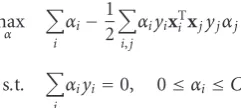
During training, an SVM solves the constrained quadratic optimization problem [30]
max
α
i
αi−
1 2
i,j
αiyixTixjyjαj
s.t.
i
αiyi=0, 0≤αi≤C,
(11)
whose solution is a vector of coefficientsαi that measure
the information content of the examples and are nonzero only for the support vectors. The coefficients are prescribed not to exceed the capacityC, which limits the influence of potentially problematic points on the final result.
The projection to higher dimensions occurs by substitut-ing the scalar products
xT
ixj−→K
xi,xj
≡φxi
T
φxj
(12)
for some mapping φ(x). The functionK is the kernel we mentioned earlier. It is not necessary to knowφto findK: any function that combines two vectors into a scalar and fulfills the (not very restrictive) set of conditions spelled out in Mercer’s theorem [31] can be used as a kernel. Some kernels stretch out the examples into the added dimensions in such a way that gaps open up between the examples which permit a flat separating surface to pass through. In this paper, we use the radial basis function (RBF) kernel
Kxi,xj
=exp
⎛ ⎜
⎝−
xi−xj
T
xi−xj
2σ2
⎞ ⎟
⎠, (13)
which surrounds every example with a surface that in a sense “repels” the separating hyperplane. The Gaussian width σ is a second adjustable parameter and usually has a scale on the order of the average separation between points. In [32] it was found that polynomial kernels may outperform the RBF kernel in some electromagnetic inverse problems. We
find that the linear kernel makes similar predictions and runs faster than the RBF, though the difference in run time is negligible for the number of training data and example features that we use in this study.
Onceαis known, the SVM can predict the attribute of an unknown example using the function [29,33]
f(x)=sgn
⎛
⎝
i∈sv
αiyiK(xi,x)
⎞
⎠. (14)
There are several ways to generalize the SVM pro-cedure to perform multiclass categorization. These have been reviewed in [11], whose authors conclude that the methods more suitable for practical use perform several binary classifications instead of attempting to separate all classes at once. In this work we adopt a one-against-one approach [34] in which the system carries outk
2
=k(k−
1)/2 optimizations and obtains the same number of decision functions of the form (14). When given an example to predict, the algorithm proceeds by ballot: it evaluates the decision functions one by one on the example and adds a vote to the one category (out of two) in which it is predicted to be. At the end, the example is assigned to the category with the most votes; should there be a tie between two classes, the program arbitrarily selects that with the smallest label.
4. Results
4.1. Data Acquisition. The Camp Sibert blind-test data were collected over 216 test cells, each of which was a square plot of side 5 m and contained at most one anomaly. The targets of interest were 4.2 mortar shells like the one in
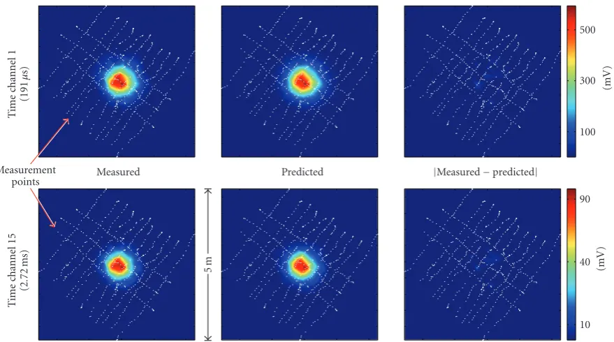
Figure 1(a), which were to be discriminated from explosion byproducts represented by the base plates and partial shells of Figures1(b)and1(c). Other sites had smaller shrapnel or non-UXO related scrap instead, and a few were essentially empty. We were given the ground truth for 66 of these cases, which we used to build a catalog of expected total NSMS values that were then tested on the 150 other cells. The EM-63 took data over 26 channels that span in approximately logarithmic fashion a lapse of time between 180μs and 25 ms. In our analysis, we use 25 of these channels, starting with the second. Measurements were taken at grids of between 400 and 700 points that crisscrossed each cell; each grid row was separated some 50 cm from its neighbors, and within each track the spacing between consecutive measurements was on the order of 5 cm. The EM-63 was always placed 30 cm above the ground.Figure 4shows a typical experimental situation, corresponding to Cell no. 7 of the study and containing 668 measurement points.
10 40 90
(mV
)
100 300 500
(mV
)
Measured Predicted |Measured−predicted|
5m
T
ime
ch
annel
1
5
(2
.
72
ms)
T
ime
ch
annel
1
(191
μ
s)
Measurement points
Figure4: A typical cell from the Camp Sibert EM-63 blind test, no. 7 in this case, consists of a square plot of side 5 m. The white dots show the measurement points distributed on a 668-point grid; the separation between rows is about 50 cm and that between consecutive points is some 5 cm. The contour plots show the measured (left column) and HAP/NSMS-predicted (middle column) near-field distributions for this cell, as well as the mismatch between the two (right column), for two time gates. The first time channel (top row) is taken 191μs after shutdown; the 15th (bottom) is centered at 2.72 ms.
plot and located 30 cm below the sensor (i.e., at ground level) and divide it into 11×11 patches, each of which is assumed to contain a magnetic-charge distribution of uniform density. We take the measured field data (as seen for example on the left column ofFigure 4) and use (5) to determineq, which in turn allows us to determineψ(r) using (7) and construct the matrices of (4) to find the location. We do this separately for every time channel and get consistent location estimates from gate to gate, which lends credence to their precision. For the case of Cell no. 7, we obtain a target depth of 55 cm, acceptably close to the ground truth of 60 cm.
To compute the NSMS amplitudeQ(t) we surround the target with a prolate spheroid with semiminor axisa=5 cm and elongatione ≡b/a = 4. This spheroid is divided into 7 azimuthal belts, each of which is assumed to contain a radial-magnetic-dipole distribution of constant density. The spheroid is placed at the location estimated by the HAP method and the orientation given by the dipole momentm
obtained from (2) and (7). With all the pieces in place, we can proceed to apply (8) to findΩand (9) to extractQ(t) for the target, which eventually reveals it as the UXO ofFigure 5(a). ThisQ(t) curve appears as a line of pentagons inFigure 3, which also depicts the resulting total NSMS values for the rest of the targets. We determine the Pasion-Oldenburg parametersk,β, andγfor each anomaly by a direct nonlinear least-squares fit of (10) and by linear (pseudo)inversion of its logarithm; both procedures gave consistent results. In general, we obtain good fits to the measured fields [4];
Figure 4shows that the discrepancy between the actual data and the model prediction runs only to a few percent.
We have previously found [3,4] that the ratio of Qat the 15th time channel toQat the first time channel, which involves a fixed superposition ofβandγ, shows discernible clustering for this particular data set when combined with the third parameterk. (The 15th time channel, centered at about 2.7 ms, was chosen because it takes place late enough to show the behavior described above but early enough that all targets still have an acceptable signal-to-noise ratio; nearby time channels produce similar results.) The values of R ≡Q(t15)/Q(t1) for the 4.2mortars are particularly well grouped and for the most part noticeably distinct from those of the others, suggesting that this two-dimensional feature space may be used to perform dependable classification. This suggestion is confirmed by our SVM analysis.
(a) Shell at no. 7 (b) Twisted chain (c) Crumpled debris
Figure 5: (a) Unexploded shell from Cell no. 7, and (b), (c) the two false alarms obtained by the SVM classifier using k and R as discriminators.
0.5 1 1.5 2 2.5 3 3.5 4 logk
−3.5
−3
−2.5
−2
−1.5
−1
−0.5
log
R
UXO Partial Base
Scrap Clutter Empty
Figure 6: Result of the SVM classification for the Camp Sibert anomalies using the logarithms ofk and R ≡ Q(t15)/Q(t1). The SVM has been trained with capacityC=10 and kernel widthσ = 1/200. The small markers denote the ground truth for both training (hollow) and testing (solid) cells. The larger markers highlight the cases where there is a disagreement between the ground truth and the SVM prediction.
SVM implementation. A more systematic search forC and γ using five-fold cross-validation [5] recommends slightly higher capacities that result in identical predictions.
ForRandk as features, we find the best SVM perfor-mance usingC = 10. The results are displayed (for testing data only) inTable 1and shown pictorially (for both training and testing) inFigure 6. The matrix elementci j in the table
denotes an item of categoryithat was identified by the SVM as belonging to category j; in other words, the rows of this contingency table correspond to the ground truth and the columns to predictions. The small markers in the plot show the ground truth (hollow for training data and filled for the
tests), while the large markers point out the items for which the SVM makes wrong predictions. For example, a small yellow upright triangle surrounded by a large cyan square is a piece of scrap (clutter unrelated to UXO) incorrectly identified as a base plate. The UXO, with their high initial amplitudes and slow decay, are clustered at the top right corner. We see that there are only two false alarms (i.e., objects identified with UXO that were in fact something else) and that all potentially dangerous items have been identified correctly.
The false alarms, two pieces of non-UXO clutter, appear on Figures 5(b) and 5(c). They are seen to be similar to the 4.2mortars in size and metal content (cf.Figure 5(a)), which makes theirkandRvalues lie closer to the tight UXO cluster than to any other anomaly inFigure 6. Here we note that, as can be seen inFigure 1(d), the training data provided by the examiners was somewhat biased toward UXO, while clutter and scrap samples were underrepresented (this was not the case with the testing data and should not be expected in future tests). If we switch training and testing data in the SVM analysis, we can achieve perfect discrimination without varying the capacity—though in this case we have more training data than tests. This highlights the importance of having a diverse collection of representative samples to use during the training stage.
We can repeat the analysis using other two-dimensional combinations of the Pasion-Oldenburg parameters. Com-bining k and γ yields results similar to those of k and R, as Figure 7 and Table 2 show. Figure 8 and Table 3
Table1: SVM classification of Camp Sibert anomalies usingkandRwithC=10.
k,R;C=10 SVM prediction
UXO Partial Base Clutter Scrap Empty
Ground truth
UXO 34 0 0 0 0 0
Partial 0 22 0 1 0 0
Base 0 0 39 1 0 0
Clutter 0 0 4 19 0 2
Scrap 2 0 3 4 13 0
Empty 0 1 1 1 2 1
Table2: SVM classification of Camp Sibert anomalies usingγandkwithC=9.
γ,k;C=9 SVM prediction
UXO Partial Base Clutter Scrap Empty
Ground truth
UXO 34 0 0 0 0 0
Partial 5 17 0 1 0 0
Base 0 0 39 0 1 0
Clutter 0 0 4 15 5 1
Scrap 2 1 3 5 11 0
Empty 1 1 2 2 0 0
0 0.5 1 1.5 2 2.5 3 3.5 4 logk
−1
−0.5 0 0.5 1 1.5 2
log
γ
UXO Partial Base
Scrap Clutter Empty
Figure 7: Result of the SVM classification for the Camp Sibert anomalies using the logarithms of the Pasion-Oldenburg parame-terskandγ. The SVM here has a capacityC=9. The small markers denote the ground truth for both training (hollow) and testing (solid) cells. The larger markers show the wrong SVM predictions.
It is helpful and straightforward to increase the dimen-sionality of the feature space. Figure 9shows the discrimi-nation obtained by running the SVM using all three Pasion-Oldenburg features. The capacityC=9 here, and increasing it changes the results only slightly. The number of false alarms increases: we get the same two pieces of scrap from before, and now a few of the partial mortars are identified as UXO by the algorithm, due in part to the small range ofβ
−1 −0.5 0 0.5 logβ
−1
−0.5 0 0.5 1 1.5 2
log
γ
UXO Partial Base
Scrap Clutter Empty
Figure 8: Result of the SVM classification for the Camp Sibert anomalies using the logarithms of the Pasion-Oldenburg parame-tersβandγ. The SVM capacityC=105. The small markers denote the ground truth for both training (hollow) and testing (solid) cells. The larger markers highlight the wrong predictions made by the SVM.
and in part to the large gap between the UXO and the other anomalies, clearly visible in the figure, which again calls out for more and more-diverse training information.
Finally, it is possible to dispense with the Pasion-Oldenburg model altogether and run an SVM using the “raw”Q(t) as input. The feature space has dimensionality
Table3: SVM classification of Camp Sibert anomalies usingγandβwithC=105.
γ,β;C=105 SVM prediction
UXO Partial Base Clutter Scrap Empty
Ground truth
UXO 34 0 0 0 0 0
Partial 0 14 5 2 1 1
Base 3 0 37 0 0 0
Clutter 0 1 5 14 1 4
Scrap 3 1 1 3 13 1
Empty 2 0 0 3 1 0
Table4: SVM classification of Camp Sibert anomalies using allQvalues (scaled byQ(t1)) withC=20.
Q/Q(t1);C=20 SVM prediction
UXO Partial Base Clutter Scrap Empty
Ground truth
UXO 34 0 0 0 0 0
Partial 0 15 0 7 1 0
Base 3 0 34 3 0 0
Clutter 0 2 3 14 4 2
Scrap 3 1 3 3 12 0
Empty 2 2 1 0 1 0
Table5: SVM classification of Camp Sibert anomalies using allQvalues (unscaled) withC=1.
AllQ;C=1 SVM prediction
UXO Partial Base Clutter Scrap Empty
Ground truth
UXO 34 0 0 0 0 0
Partial 5 17 0 1 0 0
Base 0 0 39 0 1 0
Clutter 0 2 4 18 1 0
Scrap 2 2 3 2 13 0
Empty 0 1 1 2 2 0
the results. The performance is slightly inferior to that of Rversusk; the usual two false alarms are there, along with a few new ones. All the UXO are identified correctly. We can also use the logarithm ofQwithout any scaling (though the SVM internally rescales the feature space to [0, 1]Δ). A capacityC=1 suffices here. The results appear onTable 5. All dangerous items are once more identified as such.
5. Conclusion
In this paper, we have applied the NSMS model to EM-63 Camp Sibert discrimination data sets. First the locations of the objects were inverted for by the fast and accurate dipole-inspired HAP method. Subsequently, each anomaly was characterized at each time channel through its total NSMS strength. Discrete intrinsic features were selected and extracted for each object using the Pasion-Oldenburg decay law and then used as input for a support vector machine that classified the items.
Our study reveals that the ratio of an object’s late response to its early response can be used as a robust discriminator when combined with the Pasion-Oldenburg amplitude k. Other mixtures of these parameters also result in good classifiers. Moreover, we can use Qdirectly, completely obviating the need for the Pasion-Oldenburg fit. In each case, the classifier runs by itself and does not require any human intervention. The SVM can be trained very quickly, even when the feature space has more than 20 dimensions, and it is a simple matter to add more training data on-the-fly. It is also possible to use already processed data to classify examples as yet unseen.
4
1 2
3
5 logk
1 2
logγ
−1
−2 logβ
UXO Partial Base
Scrap Clutter Empty
Figure9: SVM classification of the Camp Sibert anomalies using the logarithms ofk, β, andγ. The SVM hasC = 9. The small markers denote the ground truth for both training and testing cells. The larger markers highlight the cases where there is a disagreement between the ground truth and the SVM prediction.
false alarms come to be: some of the clutter items have a response that closely resembles that of UXO. While this will inevitably arise, it may still be possible to make the SVM more effective—and perhaps get close to reaching 100% accuracy—by including some of these refractory cases during the training. That said, there will certainly be cases in the field where the nonuniqueness inherent to noisy inverse scattering problems will cause the whole procedure to fail and yield dubious estimates. In those cases it will be necessary to assume the target is dangerous and dig it out.
In a completely realistic situation, where in principle no training data are given and the ground truth can be learned only as the anomalies are excavated, one can never be sure that the data already labeled constitute a representative sample containing enough of both dangerous and innocuous items. This difficulty is mitigated by two facts: (1) usually at the outset we have some idea of the kind of UXO present in the field and (2) the (usually great) majority of detected anomalies will not be UXO and thus random digging will produce a varied sampling of the clutter present. Methods involvingsemisupervised learning exploit this gradual revealing of the truth and have been found to perform better at UXO discrimination than supervised learning methods like SVM when starting from the point dipole model [35,36]. (Activelearning methods, which try to infer which anomalies would contain the most useful
information and could thus serve to guide the anomaly unveiling, show further, though fairly minor, improvement.) Combining this more powerful learning procedure with the excellent performance of the HAP/NSMS method may enhance the discrimination protocol and should be the subject of further research.
In summary, the results presented here show that our search and characterization procedure, whose effectiveness is apparent from several recent studies [3, 4, 37, 38], can be combined with an SVM classifier to produce a UXO discrimination system capable of correctly singling out dangerous items from among munitions-related debris and other natural and artificial clutter. In future investigations, we will continue to hone these algorithms and use them on other blind tests, including some already carried out in saltwater instead of soil.
Acknowledgment
This work was supported by the Strategic Environmental Research and Development Program through Grants no. MM-1572 and no. MM-1573.
References
[1] J. Byrnes, Ed.,Unexploded Ordnance Detection and Mitigation, NATO Science for Peace and Security Series B: Physics and Biophysics, Springer, Dordrecht, The Netherlands, 2009. [2] J. D. McNeill and M. Bosnar, “Application of TDEM
tech-niques to metal detection and discrimination: a case history with the new Geonics EM-63 fully time-domain metal detec-tor,” Tech. Rep. TN-32, Geonics LTD, Mississauga, Canada, 2000,http://www.geonics.com/.
[3] F. Shubitidze, J. P. Fern´andez, B. E. Barrowes, I. Shamatava, and K. O’Neill, “Normalized surface magnetic source model applied to camp sibert data: discrimination studies,” in Proceedings of the Applied Computational Electromagnetics Symposium (ACES ’09), Monterey, Calif, USA, March 2009. [4] F. Shubitidze, J. P. Fern´andez, I. Shamatava, L. R. Pasion, B. E.
Barrowes, and K. O’Neill, “Application of the normalized sur-face magnetic source model to a blind unexploded ordnance discrimination test,”Applied Computational Electromagnetics Society Journal, vol. 25, no. 1, pp. 89–98, 2010.
[5] C.-C. Chang and C.-J. Lin, “LIBSVM: a library for sup-port vector machines,” 2009, http://www.csie.ntu.edu.tw/∼ cjlin/libsvm/.
[6] B. E. Boser, I. M. Guyon, and V. N. Vapnik, “A training algorithm for optimal margin classifiers,” in Proceedings of Annual 5th ACM Workshop on Computational Learning Theory, D. Haussler, Ed., pp. 144–152, ACM Press, London, UK, 1992.
[7] V. N. Vapnik, “An overview of statistical learning theory,”IEEE Transactions on Neural Networks, vol. 10, no. 5, pp. 988–999, 1999.
[8] V. Cherkassky and F. Mulier, Learning from Data: Concepts, Theory, and Methods, John Wiley & Sons, New York, NY, USA, 1998.
[10] A. J. Smola and B. Sch¨olkopf, “A tutorial on support vector regression,”Statistics and Computing, vol. 14, no. 3, pp. 199– 222, 2004.
[11] C.-W. Hsu and C.-J. Lin, “A comparison of methods for multiclass support vector machines,” IEEE Transactions on Neural Networks, vol. 13, no. 2, pp. 415–425, 2002.
[12] Y. Zhang, L. Collins, H. Yu, C. E. Baum, and L. Carin, “Sensing of unexploded ordnance with magnetometer and induction data: theory and signal processing,” IEEE Transactions on Geoscience and Remote Sensing, vol. 41, no. 5, part 1, pp. 1005– 1015, 2003.
[13] J. P. Fern´andez, B. Barrowes, K. O’Neill, et al., “Evaluation of SVM classification of metallic objects based on a magnetic-dipole representation,” in Detection and Remediation Tech-nologies for Mines and Minelike Targets XI, J. T. Broach, R. S. Harmon, and J. H. Holloway Jr., Eds., vol. 6217 ofProceedings of SPIE, Bellingham, Wash, USA, April 2006.
[14] X. Chen,Inverse problems in electromagnetics, Ph.D. disserta-tion, Massachusetts Institute of Technology, Cambridge, Mass, USA, June 2005.
[15] B. Zhang, K. O’Neill, J. A. Kong, and T. M. Grzegorczyk, “Support vector machine and neural network classification of metallic objects using coefficients of the spheroidal MQS response modes,”IEEE Transactions on Geoscience and Remote Sensing, vol. 46, no. 1, pp. 159–171, 2008.
[16] J. P. Fern´andez, K. Sun, B. Barrowes, et al., “Inferring the location of buried UXO using a support vector machine,” in Detection and Remediation Technologies for Mines and Minelike Targets XII, R. S. Harmon, J. T. Broach, and J. H. Holloway Jr., Eds., vol. 6553 ofProceedings of SPIE, pp. 65530B.1–65530B.9, Bellingham, Wash, USA, April 2007.
[17] A. Massa, A. Boni, and M. Donelli, “A classification approach based on SVM for electromagnetic subsurface sensing,”IEEE Transactions on Geoscience and Remote Sensing, vol. 43, no. 9, pp. 2084–2093, 2005.
[18] E. Bermani, A. Boni, S. Caorsi, and A. Massa, “An innovative real-time technique for buried object detection,”IEEE Trans-actions on Geoscience and Remote Sensing, vol. 41, no. 4, pp. 927–931, 2003.
[19] S. Caorsi, D. Anguita, E. Bermani, A. Boni, M. Donelli, and A. Massa, “A comparative study of NN and SVM-based elec-tromagnetic inverse scattering approaches to on-line detection of buried objects,” Applied Computational Electromagnetics Society Journal, vol. 18, no. 2, pp. 65–75, 2003.
[20] A. B. Tarokh, E. L. Miller, I. J. Won, and H. Huang, “Statistical classification of buried objects from spatially sampled time or frequency domain electromagnetic induction data,”Radio Science, vol. 39, no. 4, Article ID RS4S05, 2004.
[21] A. Aliamiri, J. Stalnaker, and E. L. Miller, “Statistical classifi-cation of buried unexploded ordnance using nonparametric prior models,” IEEE Transactions on Geoscience and Remote Sensing, vol. 45, no. 9, pp. 2794–2806, 2007.
[22] I. Shamatava, F. Shubitidze, B. Barrowes, J. P. Fern´andez, L. R. Pasion, and K. O’Neill, “Applying the physically complete EMI models to the ESTCP camp sibert pilot study EM-63 data,” in Detection and Sensing of Mines, Explosive Objects, and Obscured Targets XIV, R. S. Harmon, J. T. Broach, and J. H. Holloway Jr., Eds., vol. 7303 ofProceedings of SPIE, pp. 73030O1–73030O-11, Bellingham, Wash, USA, May 2009.
[23] F. Shubitidze, D. Karkashadze, B. Barrowes, I. Shamatava, and K. O’Neill, “A new physics-based approach for estimating a buried object’s location, orientation and magnetic polariza-tion from EMI data,”Journal of Environmental and Engineering Geophysics, vol. 13, no. 3, pp. 115–130, 2008.
[24] F. Shubitidze, K. O’Neill, B. E. Barrowes, et al., “Application of the normalized surface magnetic charge model to UXO discrimination in cases with overlapping signals,”Journal of Applied Geophysics, vol. 61, no. 3-4, pp. 292–303, 2007. [25] L. R. Pasion and D. W. Oldenburg, “A discrimination
algo-rithm for UXO using time domain electromagnetics,”Journal of Environmental & Engineering Geophysics, vol. 6, pp. 91–102, 2001.
[26] A. G. Kyurkchan, B. Y. Sternin, and V. E. Shatalov, “Singular-ities of continuation of wave fields,”Physics-Uspekhi, vol. 39, no. 12, pp. 1221–1242, 1996.
[27] R. Zaridze, G. Bit-Babik, K. Tavzarashvili, D. P. Economou, and N. K. Uzunoglu, “Wave field singularity aspects in large-size scatterers and inverse problems,”IEEE Transactions on Antennas and Propagation, vol. 50, no. 1, pp. 50–58, 2002. [28] M. A. Aizerman, E. M. Braverman, and L. I. Rozonoer,
“Theoretical foundations of the potential function method in pattern recognition learning,” Automation and Remote Control, vol. 25, pp. 821–837, 1964.
[29] C. J. C. Burges, “A tutorial on support vector machines for pattern recognition,”Data Mining and Knowledge Discovery, vol. 2, no. 2, pp. 121–167, 1998.
[30] O. L. Mangasarian and D. R. Musicant, “Lagrangian support vector machines,”Journal of Machine Learning Research, vol. 1, no. 3, pp. 161–177, 2001.
[31] J. Mercer, “Functions of positive and negative type and their connection with the theory of integral equations,” Philosophical transactions of the Royal Society of London. Series A, vol. 209, pp. 415–446, 1909.
[32] E. Bermani, A. Boni, A. Kerhet, and A. Massa, “Kernels evalua-tion of SVM-based estimators for inverse scattering problems,” The phenomenon of resonance radiation of electromagnetic Research, vol. 53, pp. 167–188, 2005.
[33] N. Cristianini and J. Shawe-Taylor,An Introduction to Support Vector Machines and other Kernel-Based Learning Methods, Cambridge University Press, Cambridge, UK, 2000.
[34] U. Kreßel, “Pairwise classification and support vector machines,” in Advances in Kernel Methods: Support Vector Learning, B. Sch¨olkopf, J. C. Burges, and A. J. Smola, Eds., pp. 268–255, MIT Press, Cambridge, Mass, USA, 1999.
[35] Y. Zhang, X. Liao, and L. Carin, “Detection of buried targets via active selection of labeled data: application to sensing subsurface UXO,”IEEE Transactions on Geoscience and Remote Sensing, vol. 42, no. 11, pp. 2535–2543, 2004.
[36] Q. Liu, X. Liao, and L. Carin, “Detection of unexploded ordnance via efficient semisupervised and active learning,” IEEE Transactions on Geoscience and Remote Sensing, vol. 46, no. 9, pp. 2558–2567, 2008.
[37] F. Shubitidze, B. Barrowes, I. Shamatava, J. P. Fern´andez, and K. O’Neill, “APG UXO discrimination studies using advanced EMI models and TEMTADS data,” inDetection and Sensing of Mines, Explosive Objects, and Obscured Targets XIV, R. S. Harmon, J. T. Broach, and J. H. Holloway Jr., Eds., vol. 7303 ofProceedings of SPIE, Bellingham, Wash, USA, May 2009. [38] I. Shamatava, F. Shubitidze, B. Barrowes, J. P. Fern´andez, and