Volume 2010, Article ID 105476,11pages doi:10.1155/2010/105476
Research Article
Marker-Based Human Motion Capture in Multiview Sequences
Cristian Canton-Ferrer, Josep R. Casas, and Montse Pard `as
Signal Theory and Communications Department (TSC), Universitat Polit`ecnica de Catalunya (UPC), Campus Nord, Edif. D5, Jordi Girona 1-3, 08034 Barcelona, Spain
Correspondence should be addressed to Cristian Canton-Ferrer,[email protected]
Received 24 March 2010; Accepted 6 November 2010
Academic Editor: Jar Ferr Yang
Copyright © 2010 Cristian Canton-Ferrer et al. This is an open access article distributed under the Creative Commons Attribution License, which permits unrestricted use, distribution, and reproduction in any medium, provided the original work is properly cited.
This paper presents a low-cost real-time alternative to available commercial human motion capture systems. First, a set of distinguishable markers are placed on several human body landmarks, and the scene is captured by a number of calibrated and synchronized cameras. In order to establish a physical relation among markers, a human body model is defined. Markers are detected on all camera views and delivered as the input of an annealed particle filter scheme where every particle encodes an instance of the pose of the body model to be estimated. Likelihood between particles and input data is performed through the robust generalized symmetric epipolar distance and kinematic constrains are enforced in the propagation step towards avoiding impossible poses. Tests over the HumanEva annotated data set yield quantitative results showing the effectiveness of the proposed algorithm. Results over sequences involving fast and complex motions are also presented.
1. Introduction
Accurate retrieval of the configuration of an articulated structure from the information provided by multiple cam-eras is a field that found numerous applications in the recent years. The grown of computer graphics technology together with human motion capture (HMC) systems have been extensively used by the cinematographic and video games industry to generate virtual avatars [1]. Medicine also benefited from these advances in the field of orthopedics, locomotive pathologies assessment, or sports performance improvement [2]. In this field, despite markerless HMC systems have attained significant performance ratios in some scenarios [3], only HMC systems aided by markers placed on some body landmarks can produce high-accuracy results.
Depending on the type of employed markers, HMC sys-tems are classified in two groups: nonoptical (inertial, mag-netic, and mechanic) or optical systems (active and passive). Optical systems based on photogrammetric methods are more used than the nonoptical ones, usually requiring special suits embedding rigid skeletal-like structures [4], magnetic [5] or accelerometric devices [6] or multisensor fusion algorithms [7]. Instead, image-based or optical systems allow a relative freedom of movement and are less intrusive.
A common issue of all optical and nonoptical systems is the fact that they are usually expensive and require a dedicated hardware. The most usual involve IR retro-reflective markers that reflect back light, that is, generated near the cameras lens [8]. Other optical systems triangulate positions by using active markers that emits a pulse modulated signal. This allows distinguishing among markers and to automatically label them [9].
model. Commercial tools that perform this transformation are generally semiautomatic, thus becoming a labor-intensive task.
Once the 3D marker positions are obtained, it is required to fit a selected human body model (HBM) to these data to obtain kinematically meaningful parameters to perform either an analysis (i.e., for gesture recognition) or a synthesis (i.e., for avatar animation). However, in most of the systems, the markers’ 3D position estimation and the fitting steps are decoupled. One of the first attempts to use an anatomical human model to increase the robustness of a HMC system is presented in [11] were the algorithm computes a skeleton-and-marker model using a standardized set of motions and uses it to resolve the ambiguities during the 3D reconstruction process. Another approach using a HBM and data clustering is presented in [4]. Detection of 2D markers in separate images and its analysis using calibration information have been presented in [12] enforcing an HBM afterwards. A similar technique using a Kalman filter involving the HBM in the data association step was presented in [2].
In this paper, a low-cost real-time multicamera algorithm for marker-based human motion capture is presented. The proposed algorithm can work with any marker type detectable onto a set of 2D planes under perspective projection and it is robust to markers’ occlusion and noisy detections. Since variables involved with the employed analysis HBM do not hold a linear relationship and the involved statistical distributions are non-Gaussian, we opted for a Monte Carlo approach to estimate the pose of the HBM at a given time instant. In our case, marker detection and HBM pose estimation are performed in the same analysis loop by means of an annealed particle filter [13]. Epipolar geometry is exploited in the particle likelihood evaluation by means of the symmetric epipolar distance [14] being robust to noisy marker detections and occlusions. Moreover, kinematic restrictions are applied in the particle propagation step towards avoiding impossible poses. Finally, effectiveness of the proposed algorithm is assessed by means of objective metrics defined in the framework of the HumanEva data set [3]. The presented algorithm is intended to work with any multicamera setup and regardless of the complexity of the selected human body model.
2. Monte Carlo-Based Human Motion Capture
2.1. Problem Formulation. The evolution of a physical artic-ulated structure can be better captured with model-based tracking techniques [15]. In this process, the pose of an articulated HBM is sequentially estimated along time using video data from a number of cameras. Let y be the state vector to be estimated formed by the defining parameters of an articulated HBM, angles at every joint, andY⊂RD the state space describing all possible valid poses an HBM may adopt, wherey∈Y.
From a Bayesian perspective, the articulated motion estimation and tracking problem is to recursively estimate a certain degree of belief in the state vectorytat timet, given
the dataz1 :tup to timet. Thus, it is required to calculate the posteriorpdf p(yt | z1 :t). However, thispdf may be peaky and far from being convex, and hence cannot be computed analytically unless linear-Gaussian models are adopted. Even though Kalman filtering provides the optimal solution under certain assumptions, it tends to fail when the estimated probability density presents a multimodal distribution or the dimension of the state vector is high. Usually, this is the type ofpdfs involved in HMC processes.
2.2. Particle Filtering. Particle Filtering (PF) [16] algorithms are sequential Monte Carlo methods based on point mass (or “particle”) representations of probability densities. These techniques are employed to tackle estimation and tracking problems where the pdfs of the involved variables do not hold Gaussianity uncertainty models, linear dynamics and exhibit multimodal distributions. In this case, PF expresses the belief about the system at timetby approximating the posterior probability distribution p(yt | z1 :t), yt ∈ Y. This distribution is represented by a weighted particle set {(ytj,πtj)}Npj=1, which can be interpreted as a sum of Np Dirac functions centered on theytjwith their associated real, nonnegative weightsπtj:
py|zt
≈
Np
j=1
πtjδ
yt−ytj
. (1)
In order to ensure convergence, weights must fulfill the normalization condition jπtj = 1. For this type of estimation and tracking problems, it is a common approach to employ a Sampling Importance Resampling-(SIR)-based strategy to drive particles along time [17]. This assumption leads to a recursive update of the weights as
πtj∝πtj−1p
zt|ytj
. (2)
SIR PF circumvents the particle degeneracy problem by resampling with replacement at every time step [16]. That is, to dismiss the particles with lower weights and proportionally replicate those with higher weights. In this case, weights are set toπtj−1=Np−1, for all j, therefore
πtj∝p
zt|ytj
. (3)
Hence, the weights are proportional to the likelihood function that will be computed over the incoming datazt.
The best state at time t, Yt, is derived based on the discrete approximation of (1). The most common solution is the Monte Carlo approximation of the expectation
Yt=E p
y|zt
=
Np
j=1
πtjytj. (4)
bias the estimation. In order to cope with such cases, the estimation is set to be the state vector associated to the maximum or the mean of all particle weights. Finally, a propagation model is adopted to add a drift to the state of the re-sampled particles in order to progressively sample the state space in the following iterations [16].
Another issue arising when applying PF techniques to computer vision problems is to derive a valid observation model p(zt |ytj) relating the input datazt with the particle state ytj. Nevertheless, even if such likelihood model can be defined, its evaluation may be very computationally inefficient. Instead of that, a fitness function w(zt,ytj) :
Y → [0, 1] can be constructed according to the likelihood function, such that it provides a good approximation of p(zt|ytj) but is also relatively easy to calculate.
2.3. Annealing Strategy. PF is an appropriate technique to deal with problems where the posterior distribution is multi-modal. This usually happens when state space dimensionality is high, like in HMC. To maintain a fair representation of p(yt | z1 :t), a certain number of particles is required in order to find its global maxima instead of a local one. It has been proved in [18] that the amount of particles required by a standard PF algorithm to achieve a successful tracking follows an exponential law with the number of dimensions. Articulated motion tracking typically employs state spaces with dimensionD > 25, thus standard PF turns out to be computationally unfeasible.
There exist several possible strategies to reduce the complexity of the problem based on refinements and vari-ations of the seminal PF idea. Partitioned and hierarchical sampling [18,19] are presented as highly efficient solutions to this problem. In the instance when there exists a tractable substructure between some variables of the state model, specific states can be marginalized out of the posterior, leading to the family of Rao-Blackwellized PF algorithms [20]. However, these techniques impose a linear hierarchy of sampling which may not be related to the true body structure assuming certain statistical independence among state variables. Finally, annealed PF [13] is one of the most general and robust approaches to estimation problems involving high-dimensional and multimodal state spaces. In this work, this technique will be extended to our marker-based scenario.
Likelihood functionsw(zt,y) involved in HMC problems may contain several local maxima. Therefore, if using a single weighting function, a PF would require a large number of particles to properly sample the state space. By using annealing combined with PF, a series of weighting functions {wm(zt,y)}Ln=1 are constructed where wm+1(zt,y) slightly
differs fromwn(zt,y) and represents a smoothed version of it. In our case,wL(zt,y) is designed to be a coarse smooth version of w1(zt,y) and, typically, wm(zt,y) functions are constructed by using
wn
zt,y
=wzt,y
βn
, (5)
where βL < · · · < β1 = 1 are the annealing scheduling
parameters.
When a new measurement zt is available an annealing iteration is performed. Every annealing run consists of L steps or annealing layers where, in each of them, the appropriate weighting function is used and a set of pairs is constructed {(ynj,t,πnj,t)}
Np
j=1. Starting with an initialized
particle set{(yLj,t,πLj,t=Np−1)}Npj=1, the annealing process for
every layerncan be summarized as the following. (1) Calculate the weights:
πnj,t∝w
zt,ynj,t
βn
, (6)
enforcing the normalization conditionjπnj,t = 1. The estimation of parameter βn is based on the particle survival technique described in [13]. Once the weighted set is constructed, it will be used to draw the particles of the next layer.
(2) Resampling: draw Np particles with replacement from the set{(ynj,t,πnj,t)}
Np
j=1with distribution p(y =
ynj,t)=πnj,t.
(3) Construct the particle set corresponding to layern−1 as
ynj−1,t=y j
n,t+N(0,Σn), πnj−1,t=Np−1,
(7)
whereN(µ,Σn) stands for a truncated multivariate Gaussian distribution with mean µ and covari-ance matrix Σn that will be further described in
Section 3.5. This process is repeated until reaching n=1.
Finally the estimated stateYtis computed as
Yt=
Np
j=1
π1,jty j
1,t. (8)
The unweighted particle set for the next observation is defined as
yLj,t+1=y
j
1,t+N(0,Σ0), (9)
where the covariance matrix Σ0 is set proportional to the
maximum variation of the defining model parameters and Σn=αL−mΣ0. Settingα=0.6 provided satisfactory results. A
visual example of the annealed PF is depicted inFigure 1.
3. Filter Implementation
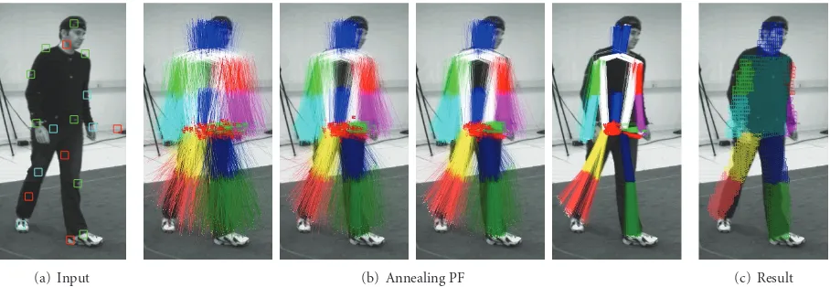
When implementing an annealed PF, several issues must be addressed: initialization, likelihood evaluation, particle propagation, and occlusion management. In the following section, we discuss the implementation of these two factors when employing a set of marker detections in multiple cameras as the input and an HBM as the tool to drive the physical relations among the variables of the state space (see
(a) Input (b) Annealing PF (c) Result
Figure1: Annealed PF operation example. (a) The output of the employed marker detector where color boxes stand for correct (green), false (red), and missed (blue) detections. (b) The progressive fitting of particles driven by the annealing process and, (c) The final pose estimation
Yt.
3.1. Initialization. In the current scenario, it is supposed that the subject under study is tracked since the moment he/she enters the scene. A simple person tracking system is employed [21] to obtain a coarse estimation of person’s position and velocity. Assuming that backward motions are unlikely, the velocity vector allows an initial estimation of the torso orientation. Finally, for the rest of limbs, a neutral and natural walking position is defined for the initialization of the HMC system.
In the case of a global miss of the tracked subject, the variance of the state space variables associated to every particle tend to be high in comparison of the variance obtained during a correct tracking operation. Therefore, the analysis of this variance allows detecting when the HMC system is out of track. In such case, the coarse tracking system is employed to start again the initialization loop described beforehand.
Although a beforehand selected HBM is employed to track any person, the size of the limbs must be adequate to the particular subject under study. For the majority of people, there is a strong quasilinear correlation between the height of a person and the length of the limbs [22] thus allowing a proper scaling of these magnitudes after automatically measuring the height directly from the input images as shown, for instance, in [14].
3.2. Measurement Generation. The input data zt to the proposed tracking system will be the detection of the 2D projections of the set of distinguishable markers attached to the body of the performer onto theNC available images
in contrast with markerless HMC systems relying on image features such as edges or silhouettes [13]. Let Dn = {d1,d2,. . .,dQn}be the set ofQn locations detected in the image captured in thenth view,In, 1 ≤ n ≤ NC. In order to generate Dn, a generic marker detection algorithm Γ : In → Dn is employed whose performance is assessed by the detection rate (DR), the false positive rate (FP), and the variance estimation error (σ2
Γ). This formulation of Γwill
allow performance comparisons of the tracking algorithm
when using different marker detection algorithms and the assessment of occlusions.
Markers are usually placed at the joints, the end of the limbs, the top of the head and the chest of the subject. The proposed method is general enough to be applied to any type of markers detectable onto a set of 2D planes under perspective projection. An example of the detections obtained by our color-based marker detection is shown in
Figure 2(b).
3.3. Likelihood Evaluation. In order to evaluate the likelihood between the body pose represented by a given particle state ytj ∈ Y with reference to the input data zt = {Dn}NCn=1,
a fitness function w(zt,ytj) must be defined. The M 3D positions of the HBM landmarks corresponding to the pose described by the state vector ytj are computed through forward kinematics [12]. Let us denote these coordinates as the setX = {x1,x2,. . .,xM},xm ∈ R3. The fitness function relating the 3D locations set X with the 2D observations {Dn}NCn=1 should measure how well these 2D points fit as
projections of the setX. A similar problem was tackled by the authors in [14] in a Bayesian framework and the underlying idea is applied in this context.
For every element xm ∈ X, its projection onto every camera is computed as
pm,n=Pnxm, 1≤n≤NC, (10)
wherePn∈M4×3is the projection matrix associated to the
nth camera [10] and tilde denotes homogeneous coordinates. Then, the setTm = {t1,t2,. . .,tNC} containing the closest
measurement in every camera view for every HBM landmark xmis constructed as follows:
tn= min dq∈Dn
pm,n−dq, ∀n. (11)
x
x
x
y
y
y
y x
y z
z
z
(a) (b)
Figure2: Human body model and measurement examples. In (a), the HBM employed in this paper is parameterized as follows: 2 DOF in the neck, 3 DOF in the shoulders, 1 DOF in the elbows, 3 DOF in the hips, 3 in the lower torso and 1 DOF in the knee. Red dots mark the HBM landmarks that can be computed by applying forward kinematics. In (b), the output of the employed color based marker location detection algorithm. Colors describe the correct detections (green), the miss detections (blue) and the false positive detections (red). All this detections will conform the measurement setDn.
marker detection algorithm. In order to detect such cases, a thresholding is applied to the elementstndismissing those measurements above a threshold ρ. In this case, tn = ∅ using an empirically determined value of ρ = 10 pixels. At this point, it is required measure how likely are the set of 2D measurementsTm to be projections of the 3D HBM landmarkxm. This can be done by means of the generalized symmetric epipolar distancedSE(·) [14].
Letl(xi,j) be the epipolar line generated by the pointx in a given viewi onto another view j. Symmetric epipolar distance between two pointsdSE(xi,xj), in the two viewsi,j, is defined as
dSE
xi,xj
d2lxi,j,xj+d2(l(xj,i),xi), (12)
where d(l(xi,j),xj) is defined as the Euclidean distance between the epipolar linel(xi,j) and the pointxjas depicted inFigure 3. The extension of the symmetric epipolar distance fork≥2 points (inkdifferent views)dSE(x1,. . .,xk) can be written in terms of the distance defined in (12) as [14]
dSE
x1,. . .,xk= k
−1
i=1
k
j=i+1
d2
SE(xi,xj). (13)
This distance produces low values when the 2D points are coherent, that is, when they are projections of the same 3D location. The scoresmassociated toTm, and therefore toxm, is defined as
sm
zt,ym
≡sm(zt,Tm)∝dSEt1,t2,. . .,tNC
, (14)
View from cam 0 View from cam 1
l(x1
, 0)
d(l(x1, 0),x0) d(l(x0, 1),x1)
x0 l(x0, 1)
x1
Figure 3: Symmetric epipolar distance between two points
dSE(x0,x1).
and normalized such that sm(zt,Tm) ≤ 1. In the case where the nonempty elements ofTmis below 2, the distance dSE(Tm) cannot be computed. Under these circumstances, we setsm(zt,Tm)=1.
Assuming that the involved errors follow a Gaussian distribution [23], an accurate way to define the weighting functionw(zt,y) is
wzt,y
=exp
⎛ ⎝−1
M M
m=1
sm(zt,xm)
⎞
⎠. (15)
there areMmarkers attached to some HBM landmarks, the setDnwould ideally contain theMn≤M2D projections of the markers that are not affected by the occlusions produced by the body itself onto thenth camera view. Moreover, there might be some miss-detections of these projection and a number of false measurements.
Within the current analysis framework, occlusions and miss-detections can be assumed as an underperformance of the generic marker detectionΓthus regarded by the miss-detection rate DR. As previously noted, the amount of false positives is represented by the false positive rate FP and the error committed in the marker location estimation is assumed to have a Gaussian distribution with variance σ2
Γ.
This formation will allow simulating an arbitrary degree of corruption of the input data, as will be shown inSection 4.
Markers that are visible in, at least, three camera views can be correctly handled by the likelihood function. In the case of severe occlusions where there are only two camera views containing projections of a given marker, the distance dSE may become inaccurate. In such cases, the position of the occluded marker is estimated using information from both the correctly estimated 3D neighboring landmarks and applying temporal coherence.
3.5. Propagation Model. Kinematic restrictions imposed by the angular limits at each joint of the HBM may produce a more robust tracking output. In this field, some methods employ large volumes of annotated data to accurately model the angular cross-dependencies among joints [24] or to learn dynamic models associated to a given action [25]. In our case, these angular constraints will be enforced in the propagation step of the APF scheme. Typically, the propagation step consists in adding a random component to the state vector of a particle as
ytj=ytj−1+N(0,Σ)=Nytj−1,Σ. (16) That is, to generate samples from a multivariate Gaussian distribution centered at ytj−1 with covariance matrix Σ.
However, this may lead to poses out of the legal angular ranges of the HBM. In order to avoid such effect, some works [26] add a term into the likelihood function that penalizes particles that do not fulfill the angular constraints. The following alternative is proposed to take into account angular constrains and draw samples from a truncated Gaussian distribution [27], denoted asNand shown inFigure 4. In this way, particles are generated always within the allowed ranges thus avoiding the evaluation of particles that encode impossible poses and therefore increasing the performance of the sampling set.
4. Experiments and Results
4.1. Synthetic Data on HumanEva. In order to test the proposed algorithm, HumanEva data set [3] has been selected since it provides synchronized and calibrated data from both several cameras and a professional motion capture (MoCap) system to produce ground truth data. This data set contains a set of 5 actions performed by 3 different subjects
captured by 4 fully calibrated cameras with a resolution of 640×480 pixels at 30 fps.
HumanEva suggests two metrics, mean,μ, and standard deviation of the estimation error, σ, towards providing quantitative and comparable results. In this paper, metrics proposed in [28] for 3D human pose tracking evaluation are also employed. Let X = {x1,x2,. . .,xM}, xm ∈ R3, denote theMlandmark positions of the HBM (typically, the body joints and the end of the limbs) corresponding to the pose described by the state variabley ∈Ycomputed using forward kinematics [12] at a given time t. Assuming that landmark positionsxmassociated to particleyjare available, we can define amatchedmarker estimationxmwith respect to the ground truth positionxmas the one fulfilling= xm−
xm < δ. This stands for those estimations that fallδ-close to the ground truth position. Then, the Multiple Marker Tracking Accuracy (MMTA) is defined as the percentage of markers xm ∈ X fulfilling the < δ condition, and the Multiple Marker Tracking Precision (MMTP) as the average of the metric error betweenxmandxm, of all pairs fulfilling < δ. Finally, these scores are averaged for all frames in the sequence. Threshold δ, being an upper-bound of the maximum allowed error, is set to δ = 100 mm in our experiments.
As it has been presented in Section 3.2, the input measurements zt of the proposed algorithm are a set of 2D detections, Dn, measured over NC cameras for every time instantt. A synthetic data generation strategy has been devised where the 2D projection of the markers onto all camera views are computed from the 3D ground truth data, noted as Xt. This process is exemplified in Figure 5 and defined as follows.
(1) Inverse kinematics are applied toXt to estimate the pose of a HBM and body parts are fleshed out with super ellipsoids.
(2) Every 3D location in Xt is projected onto every camera in order to generate the setsDn, 1≤n≤NC. The previously estimated fleshed HBM checks the visibility of markers onto a given camera view by modeling the possible auto-occlusions among body parts. At this point, the 2D locations contained in Dn are the positions obtained by an ideal marker detection algorithm.
(3) The effect of the marker detection algorithm Γ is simulated by generating a number of miss detections, false measurements and, finally, adding a Gaussian noise to all measurements, according to the statistics reflected by DR, FP, andσΓ2.
In order to test the performance of the proposed tracking algorithm, two factors must be taken into account: the performance of the marker detection algorithm Γ (deter-mined by the triplet{DR, FP,σΓ2}) and the algorithm design
θ+
yk t−1 θ−
θ
(a) (b)
Figure 4: Angular constraints enforcement by propagating particles within the allowed angular ranges [θ−,θ+]. In (a), samples are
propagated following a truncated Gaussian distributionNcentered atytj−1with covariance matrixΣ=σ bounded betweenθ− andθ+
(green zone). (b) An example of particle propagation in the knee angle displaying how propagated particles never fall out the legal ranges
(θ <0).
simulation are depicted inFigure 6where the MMTA score is displayed as the more informative metric [28].
When analyzing the impact of missing projections of markers, that is, occlusions, represented by DR and shown in
Figure 6(a), it can be seen that the algorithm is still robust producing accurate estimations even in the case of a large miss of data, DR = 0.4. Assuming a fixed and realistic amount of occlusions, DR = 0.85, we can explore the influence of the other distorting factors. Analyzing the results shown inFigure 6(b), it may be seen that the algorithm is robust against the number of false detections FP since it is very unlikely that false 2D measurements in different views keep a 3D coherence. In this case, the spacial redundancy is efficiently exploited to discard these measurements. On the other hand, the performance of the algorithm decreases as the 2D marker position estimation error increases, σ2
Γ.
Another evident fact to be emphasized is the overannealing effect. The performance of the algorithm is not monoton-ically increasing with the number of employed annealing layers. This happens when the particles concentrate too much around the peaks of the weighting function hence impoverishing the overall representation of the likelihood distribution. For this motion tracking problem, we found that the optimal configuration isL=3 andNp=700.
4.2. Real Data. The presented body tracking algorithm has been applied to capture motion figures from 4 different types of dances:salsa,belly dancing, and two Turkish folk dances. The analysis sequences were recorded with 6 fully calibrated cameras with a resolution of 1132×980 pixels at 30 fps.
Markers attached to the body of the dance performer were little yellow balls and a color-based detection algorithm Γhas been used to generate the setsDnfor every incoming multi-view frame. The original images are processed in the YCrCb color space which gives flexibility over intensity variations in the frames of a video as well as among the videos captured by the cameras from different views. In order to learn the chrominance information of the marker color, markers on the dancer are manually labeled in one frame
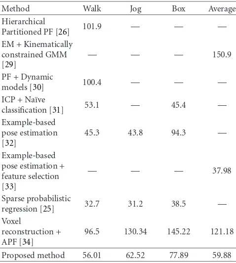
Table1: Result comparisons with state-of-the art methods evalu-ated over the HumanEva dataset. The presented score corresponds to the mean of the error estimationμ, as reported by the compared authors in their respective contributions.
Method Walk Jog Box Average
Hierarchical
Partitioned PF [26] 101.9 — — —
EM + Kinematically constrained GMM [29]
— — — 150.9
PF + Dynamic
models [30] 100.4 — — —
ICP + Na¨ıve
classification [31] 53.1 — 45.4 — Example-based
pose estimation [32]
45.3 43.8 94.3 —
Example-based pose estimation + feature selection [33]
— — — 37.98
Sparse probabilistic
regression [25] 32.7 31.2 38.5 —
Voxel
reconstruction + APF [34]
96.5 130.34 145.22 121.18
Proposed method 56.01 62.52 77.89 59.88
for all camera views. It was assumed that the distributions of Cr and Cb channel intensity values belonging to marker regions are Gaussian. Thus, the mean can be computed over each marker region (a pixel neighborhood around the labeled point). Then, a threshold in the Mahalanobis sense is applied to all images in order to detect marker locations. An empirical analysis showed that the detector Γ had the following performance triplet: DR = 0.98, FP = 4, and σ2
(a) (b) (c) (d) (e)
Figure5: Synthetic data generation process. Since the reflective markers are not distinguishable in the original RGB image (a), the sets
{Dn}NC
n=1are generated from the 3D locations provided by the MoCap system. First, for a given viewn, all 3D markers are projected onto the
corresponding image (b), and those affected by body auto-occlusions are removed (c). Then, the marker detection algorithmΓis applied: some markers are missed due to the detection ratio (d), and a number of false measurements are generated (e). Finally, an amount of Gaussian noise with varianceσ2
Γis added simulating the position estimation error.
200 400 600 800 2
4 6
200 400 600 800 2
4 6
200 400 600 800 2
4 6
200 400 600 800 2
4 6
DR=0.4 DR=0.6 DR=0.9 DR=1
(a) 2 4 6 2 4 6 2 4 6 2 4 6 2 4 6 2 4 6 2 4 6 2 4 6 2 4 6
σΓ2=0 σΓ2=20 σΓ2=40 σΓ2=60 σΓ2=80 σΓ2=100
200 400 600 800 200 400 600 800
200 400 600 800 200 400 600 800 200 400 600 800 200 400 600 800
2 4 6 2 4 6 2 4 6 2 4 6 2 4 6 2 4 6 2 4 6 2 4 6 2 4 6
200 400 600 800 200 400 600 800
200 400 600 800 200 400 600 800 200 400 600 800 200 400 600 800
2 4 6 2 4 6 2 4 6 2 4 6 2 4 6 2 4 6 2 4 6 2 4 6 2 4 6
200 400 600 800 200 400 600 800
200 400 600 800 200 400 600 800 200 400 600 800 200 400 600 800
2 4 6 2 4 6 2 4 6 2 4 6 2 4 6 2 4 6 2 4 6 2 4 6 2 4 6
200 400 600 800 200 400 600 800
200 400 600 800 200 400 600 800 200 400 600 800 200 400 600 800
2 4 6 2 4 6 2 4 6 2 4 6 2 4 6 2 4 6 2 4 6 2 4 6 2 4 6
200 400 600 800 200 400 600 800
200 400 600 800 200 400 600 800 200 400 600 800 200 400 600 800
2 4 6 2 4 6 2 4 6 2 4 6 2 4 6 2 4 6 2 4 6 2 4 6 2 4 6
200 400 600 800 200 400 600 800
200 400 600 800 200 400 600 800 200 400 600 800 200 400 600 800
FP = 100 FP = 80 FP = 60 FP = 40 FP = 20 FP = 0 (b)
Figure6: Quantitative results over the HumanEva data set where score MMTA is displayed in pseudocolor. In all plots,y-axis accounts for the number of layersLandx-axis for the number of particles per layerNp. In (a), assuming an ideal case where FP=0 andσΓ2=0, impact
of the number of occlusions, regarded by DR in the overall performance. In (b), assuming a fixed occlusion level DR=0.85, results for the cases FP= {0, 20, 40, 60, 80, 100}andσ2
(a) Salsa figures
(b) Belly dancing figures
Figure7: Dance motion tracking results. Two examples of dance tracking: salsa and belly dancing.
In this particular scenario, the algorithm had to cope with very fast motion associated to some figures. Even though these harsh conditions, the results were satisfac-tory and visually accurate as shown in Figure 7. Check
http://www.cristiancanton.org/for some example videos.
4.3. Results Comparison. A number of algorithms in the literature have been evaluated using HumanEva-I and their results have been reported in Table 1. There are two main trends in pose estimation: methods based on a tracking formulation of the problem and methods based on statistical classification. The method presented in this paper falls into the first category where some comparisons can be made. Among the reported methods, we find the expectation-maximization (EM) kinematically constrained GMM method presented by Cheng and Trivedi [29] as the continuation of the techniques already presented by Mikiˇc [35]. Addressing a complex problem such as human motion capture using EM is perhaps manageable in a benevolent scenario with well learnt constrains but, as suggested by Caillete and Howard [36] in the comparison of EM- and PF- based methods, Monte Carlo-based techniques clearly outperform those based in minimization algorithms. Other contributions reported over HumanEva-I are based on the seminal idea of PF. Husz and Wallance [26] included a particle propagation step relying on learnt information on the structure of the executed motion thus facing the already mentioned problem of lack of adaptivity to unseen motions. A very detailed dynamic model of the human kinematics is employed by Brubaker et al.[30]. Motion involving a more complex pattern such as boxing or gesturing may not cope well with these two methods.
The other family of human motion capture algorithms is based on learning and classification instead of tracking. Basically, these techniques examine the ground truth data and extract a number of features from them. Afterwards, when a new test frame is processed, these same features are extracted, and the best match between them and the already learnt ones is outputted. Results obtained with these techniques, specially those of Urtasun et al.[25] and Poppe [32], outperform the tracking-based ones. How-ever, these techniques are constrained to track a before-hand selected action and their applicability to unknown motion patterns is limited. It is notable the technique presented by M¨underman et al. [31] where a 3D recon-struction is performed before computing the features to be learnt.
To the authors knowledge, there is no evaluation of a marker-based HMC system using the HumanEva dataset. The obtained results are close to those presented by classification-based markerless methods and, although the employed input data is different, it allows qualitatively evaluating its performance. An advantage of using a marker-based method is its robustness to faulty inputs, its low complexity, and the possibility of real-time implementations.
Section 4.2usually computed directly on the camera (as done by [8]) or by the digitizing hardware.
5. Conclusion
This paper presents a robust real-time low-cost approach to marker-based human motion capture using multiple cameras synchronized and calibrated. Progressive fitting of a human body model through the annealed particle filtering algorithm using a multi-view consistency likelihood func-tion, the symmetric epipolar distance, and a kinematically constrained particle propagation model allow an accurate estimation of the body pose. Quantitative evaluation based on HumanEva dataset assessed the robustness of the algo-rithm when dealing faulty input data, even in very harsh conditions. Fast dance motion was also analyzed proving the adequateness of our technique to deal with a real scenario data.
References
[1] I. Baran and J. Popovi´c, “Automatic rigging and animation of 3D characters,” in Proceedings of the ACM International Conference on Computer Graphics and Interactive Techniques (SIGGRAPH ’07), August 2007.
[2] P. Cerveri, A. Pedotti, and G. Ferrigno, “Robust recovery of human motion from video using Kalman filters and virtual humans,”Human Movement Science, vol. 22, no. 3, pp. 377– 404, 2003.
[3] L. Sigal, A. O. Balan, and M. J. Black, “HumanEva: syn-chronized video and motion capture dataset and baseline algorithm for evaluation of articulated human motion,”
International Journal of Computer Vision, vol. 87, no. 1-2, pp. 4–27, 2010.
[4] A. G. Kirk, J. F. O’Brien, and D. A. Forsyth, “Skeletal parameter estimation from optical motion capture data,” inProceedings of IEEE Computer Society Conference on Computer Vision and Pattern Recognition (CVPR ’05), pp. 782–788, June 2005. [5] “Ascension,”http://www.ascension-tech.com/.
[6] “Moven-inertial motion capture,”http://www.moven.com/. [7] D. Roetenberg,Inertial and magnetic sensing of human motion,
Ph.D. dissertation, University of Twente, Twente, The Nether-lands, 2006.
[8] “Vicon,”http://www.vicon.com/.
[9] R. Raskar, H. Nii, B. Dedecker et al., “Prakash: lighting aware motion capture using photosensing markers and multiplexed illuminators,”ACM Transactions on Graphics, vol. 26, no. 3, Article ID 1276422, 2007.
[10] R. Hartley and A. Zisserman, Multiple View Geometry in Computer Vision, C. U. Press, 2004.
[11] L. Herda, P. Fua, R. Pl¨ankers, R. Boulic, and D. Thalmann, “Using skeleton-based tracking to increase the reliability of optical motion capture,”Human Movement Science, vol. 20, no. 3, pp. 313–341, 2001.
[12] G. Guerra-Filho, “Optical motion capture: theory and imple-mentation,”Journal of Theoretical and Applied Informatics, vol. 12, no. 2, pp. 61–89, 2005.
[13] J. Deutscher and I. Reid, “Articulated body motion capture by stochastic search,”International Journal of Computer Vision, vol. 61, no. 2, pp. 185–205, 2005.
[14] C. Canton-Ferrer, J. R. Casas, and M. Pard`as, “Towards a Bayesian approach to robust finding correspondences in
multiple view geometry environments,” in Proceedings of the 4th International Workshop on Computer Graphics and Geometric Modelling, vol. 3515 ofLecture Notes on Computer Science, pp. 281–289, 2005.
[15] T. B. Moeslund, A. Hilton, and V. Kr¨uger, “A survey of advances in vision-based human motion capture and analy-sis,”Computer Vision and Image Understanding, vol. 104, no. 2-3, pp. 90–126, 2006.
[16] M. S. Arulampalam, S. Maskell, N. Gordon, and T. Clapp, “A tutorial on particle filters for online nonlinear/non-Gaussian Bayesian tracking,”IEEE Transactions on Signal Processing, vol. 50, no. 2, pp. 174–188, 2002.
[17] N. J. Gordon, D. J. Salmond, and A. F. M. Smith, “Novel approach to nonlinear/non-gaussian Bayesian state estima-tion,”IEE Proceedings, Part F, vol. 140, no. 2, pp. 107–113, 1993.
[18] J. MacCormick and M. Isard, “Partitioned sampling, articu-lated objects, and interface-quality hand tracking,” in Proceed-ings of the European Conference on Computer Vision, pp. 3–19, 2000.
[19] J. Mitchelson and A. Hilton, “Simultaneous pose estimation of multiple people using multiple-view cues with hierarchical sampling,” inProceedings of the British Machine Vision Confer-ence, 2003.
[20] J. Madapura and B. Li, “3D articulated human body tracking using KLD-Annealed Rao-Blackwellised Particle filter,” in
Proceedings of IEEE International Conference onMultimedia and Expo (ICME ’07), pp. 1950–1953, July 2007.
[21] C. Canton-Ferrer, J. R. Casas, M. Pard`as, and R. Sblendido, “Particle filtering and sparse sampling for multi-person 3D tracking,” inProceedings of IEEE International Conference on Image Processing (ICIP ’08), pp. 2644–2647, October 2008. [22] S. L. Dockstader, M. J. Berg, and A. M. Tekalp, “Stochastic
kinematic modeling and feature extraction for gait analysis,”
IEEE Transactions on Image Processing, vol. 12, no. 8, pp. 962– 976, 2003.
[23] J. Lichtenauer, M. Reinders, and E. Hendriks, “Influence of the observation likelihood function on particle filtering performance in tracking applications,” inProceedings of the 6th IEEE International Conference on Automatic Face and Gesture Recognition (FGR ’04), pp. 767–772, May 2004.
[24] L. Herda, R. Urtasun, and P. Fua, “Hierarchical implicit surface joint limits for human body tracking,”Computer Vision and Image Understanding, vol. 99, no. 2, pp. 189–209, 2005. [25] R. Urtasun, D. J. Fleet, and P. Fua, “3D people tracking with
Gaussian process dynamical models,” inProceedings of IEEE Computer Society Conference on Computer Vision and Pattern Recognition (CVPR ’06), pp. 238–245, June 2006.
[26] Z. Husz and A. Wallance, “Evaluation of a hierarchical parti-tioned particle filter with action primitives,” inProceedings of the 2nd Workshop on Evaluation of Articulated Human Motion and Pose Estimation, 2007.
[27] J. H. Kotecha and P. M. Djuric, “Gibbs sampling approach for generation of truncated multivariate Gaussian random variables,” inProceedings of IEEE International Conference on Acoustics, Speech, and Signal Processing (ICASSP ’99), pp. 1757–1760, March 1999.
[28] C. Canton-Ferrer, J. Casas, M. Pard`as, and E. Monte, “Towards a fair evaluation of 3D human pose estimation algorithms,” Tech. Rep., Technical University of Catalonia, 2009.
Proceedings of the 2nd Workshop on Evaluation of Articulated Human Motion and Pose Estimation, 2007.
[30] M. Brubaker, D. Fleet, and A. Hertzmann, “Physics-based human pose tracking,” in Proceedings of the Workshop on Evaluation of Articulated Human Motion and Pose Estimation, 2006.
[31] L. M¨underman, S. Corazza, and T. Andriacchi, “Markerless human motion capture through visual hull and articulated icp,” inProceedings of the Workshop on Evaluation of Articulated Human Motion and Pose Estimation, 2006.
[32] R. Poppe, “Evaluating example-based pose estimation: exper-iments on the humaneva sets,” in Proceedings of the 2nd Workshop on Evaluation of Articulated Human Motion and Pose Estimation, 2007.
[33] R. Okada and S. Soatto, “Relevant feature selection for human pose estimation and localization in cluttered images,” in
Proceedings of the European Conference on Computer Vision, 2008.
[34] C. Canton-Ferrer, J. R. Casas, and M. Pard`as, “Voxel based annealed particle filtering for markerless 3D articulated motion capture,” inProceedings of the 3rd IEEE Conference on 3DTV (3DTV-CON ’09), May 2009.
[35] I. Mikiˇc,Human body model acquisition and tracking using multi-camera voxel data, Ph.D. dissertation, University of California, San Diego, Calif, USA, 2003.
[36] F. Caillette and T. Howard, “Real-time markerless human body tracking with multi-view 3-D voxel reconstruction,” in